
APPENDIX D
Review of Summer Flounder Assessments
INTRODUCTION
The quality and appropriateness of a data set can sometimes best be judged from analyses and inferences derived from it. The strengths and shortcomings in the available information become apparent by examining results (e.g., parameter estimates), associated uncertainty, and sensitivity to assumptions. To evaluate summer flounder data, a number of standard assessment and data analysis techniques were applied to ascertain which data were informative and which data may be lacking, and to examine the level of information contained in model assumptions. The model structure and assumptions add information, but the added information may be wrong, depending on how well the model and assumptions match the actual situation.
EXPLORATORY ANALYSIS
The design of the NEFSC seasonal surveys is described in Appendix C. The committee analyses presented there indicate that some efficiency may be gained by reallocating sampling effort among sample strata. This gain in efficiency depends, of course, on the current state of the fish population and may have to be revised as sampling objectives change, depending on speciesspecific sampling and management priorities. Different and changing priorities in the data collection and fisheries management for specific species may lead to conflicting objectives. Managers, scientists, and stakeholders need to identify species or species complexes of major interest and specify the relative risk associated with the uncertainty for each species.
State agencies also collect data used in the National Marine Fisheries Service (NMFS) stock assessments (see Appendix C). There may be some redundancy in these data, but other reasons (e.g., political representation, verification) may exist for continuing them. Not all the survey information included in the SAW25 Report (NEFSC, 1997) was used in the 1996 NMFS assessment. Survey data on age classes 5 and older, for example, are typically excluded from the analyses for all but the Northeast Fisheries Science Center (NEFSC) winter survey. The NEFSC winter trawl survey includes information on 5+ age classes, but these data have been available only since 1992.
Table D-1 summarizes the number of surveys per age class and year in state and federal
data sets. Coverage varies by age class and over time. Ages 1 and 5+ receive less coverage in general when compared with the middle three age classes, presumably due to the catchability characteristics of the gear employed. Some surveys are missing in the most recent years due to a time lag in availability. Information on age classes 0 and 2 through 4 will therefore have the greatest influence on the overall fit of the model because those data are the most abundant.
The log-transformed mean number per tow of summer flounder at age derived from the survey data is the relative abundance measure used by the assessment model. Trends in abundance can be seen by viewing a single age class across years as tracked by the individual surveys (NEFSC, 1997), but these trends can also be viewed in summary by examining the averaged log(CPUE+1) across surveys (see Figure D-1a, Figure D-1b and Figure D-1c). The log transformation is used to achieve stability in the variances and to facilitate contrast across the widely ranging abundance values. Such a transformation is commonly applied to fishery survey indices prior to inclusion in assessments because of the log-normal variation often seen in these indices; consequently, a log scale is the most appropriate scale on which to view these data in an exploratory analysis.
When survey-by-survey data are viewed (see Figures 4-8 in Terceiro, 1999), the NEFSC winter survey shows a much greater range in data values than the other surveys and thus must contribute a significant signal to the fit even though the length of the time series is limited. The second point, which can be seen more easily in the figures averaged across surveys (see Figure D-1a, Figure D-1b and Figure D-1c) is that the relative abundance indices may have peaked with the 1995 cohort. The trends indicated by the two observations available for the 1998 cohort go in opposite directions, creating a conflict in the data that may lead potentially to equally likely but conflicting trends in model estimates. These are important features to track in interpreting the assessment results below.
Another data set that goes into the assessment is the total catch at age (Figure D-2) representing the combined catch from the commercial and recreational fisheries. From the data available, we have no way of knowing how commercial and angling effort has changed in recent years, but the upward trend in ages 3 through 5, the slightly downward trends in age classes 1 and 2, and the significant drop in catch of age-0 fish should, in conjunction with the survey indices, determine the nature of the fit by the assessment models. Interpretation of these data is complicated by the 1992 changes under Amendment 2 to the summer flounder fishery management plan, which included an annual landings quota, a minimum size limit at 33 cm, and a minimum mesh size of 140 mm. These management actions probably influence what is seen in the combined commercial and recreational catch data. Shifts from commercial to recreational harvest also should influence the catch at age as each fishery exhibits different size and age selectivity patterns. Finally, weight at age goes into the assessment. The summer flounder weight at age has not shown any directional trends over time (Figure D-3). Thus, the dynamics exhibited in model estimates should reflect mainly the catch and relative abundance indices.
ASSESSMENT
A unified picture of the factors contributing to stock dynamics can now be developed using a system of equations linking the various components. This system of equations (a model) is derived from basic principles that are assumed to represent the system. These models add structure to the estimation process by characterizing relationships that exist among population variables (e.g., population size) and observations (e.g., catch and catch per unit effort). When using models for analysis, one should always keep in mind that (1) models are simplified representations of the system; (2) assumptions made in modeling impose a structure on the information that will influence assessment results; (3) no model works well with poor data (see NRC, 1998a); and (4) even if the data are high quality
and the assumptions are appropriate, there still might not be enough data to yield accurate and precise estimates.
TABLE D-1 Number of Surveys by Year and Age Class for Which Relative Abundance Measures are Available. (Surveys include NEFSC winter, spring, and autumn surveys, MADMF spring and fall surveys, CTDEP spring and fall surveys, RIDFW fall and fixed surveys, an NJDFW survey, and a DEDFW survey.)
|
Year |
Age 0a |
Age 1 |
Age 2 |
Age 3 |
Age 4 |
Age 5+ |
|
1982 |
4 |
1 |
2 |
3 |
3 |
0 |
|
1983 |
4 |
1 |
3 |
4 |
4 |
0 |
|
1984 |
4 |
1 |
4 |
5 |
5 |
0 |
|
1985 |
5 |
1 |
5 |
6 |
6 |
0 |
|
1986 |
5 |
1 |
5 |
6 |
6 |
0 |
|
1987 |
6 |
1 |
5 |
6 |
6 |
0 |
|
1988 |
7 |
2 |
6 |
6 |
6 |
0 |
|
1989 |
6 |
2 |
6 |
6 |
6 |
0 |
|
1990 |
7 |
3 |
7 |
6 |
6 |
0 |
|
1991 |
7 |
3 |
8 |
7 |
6 |
0 |
|
1992 |
7 |
4 |
9 |
8 |
7 |
1 |
|
1993 |
7 |
4 |
9 |
8 |
7 |
1 |
|
1994 |
7 |
4 |
9 |
8 |
7 |
1 |
|
1995 |
7 |
4 |
9 |
8 |
7 |
1 |
|
1996 |
7 |
4 |
9 |
8 |
7 |
1 |
|
1997 |
7 |
4 |
9 |
8 |
7 |
1 |
|
1998 |
6 |
4 |
9 |
8 |
7 |
1 |
|
1999 |
0 |
2 |
5 |
6 |
6 |
1 |
|
a Information on young-of-the-year fish (age 0) is available from a separate set of surveys and include data from Connecticut, Virginia, North Carolina, Maryland, New Jersey, Massachusetts, and the NEFSC. NOTE: CTDEP = Connecticut Department of Environmental Protection; DEDFW = Delaware Department of Fish and Wildlife; MADMF = Massachusetts Department of Marine Fisheries; NEFSC = Northeast Fisheries Science Center; NJDFW = New Jersey Department of Fish and Wildlife; and RIDFW = Rhode Island Department of Fish and Wildlife. |
||||||
Assessment Methodology
Three modeling approaches were applied to the summer flounder data to examine the influence of the data, model structure, and model assumptions on key assessment outputs. The approaches taken were based on the LaurecShepherd VPA method (Laurec and Shepherd, 1983; Darby and Flatman, 1994), the ADAPT method (Gavaris, 1988), and an AutoDifferentiation (AD) Model Builder implementation (Fournier, 1996) of a CAGEAN method (Deriso et al., 1985). Results from these methods were compared with results from the 1999 NMFS ADAPT assessment.
Laurec-Shepherd Virtual Population Analysis (VPA)
The Laurec-Shepherd method is an example of an ad hoc VPA tuning procedure. A number of these procedures are described in the literature and used in actual fisheries. The main characteristic of these procedures is that they accept the

FIGURE D-1a Log (CPUE+1) averaged over surveys for each age class and smoothed over time.
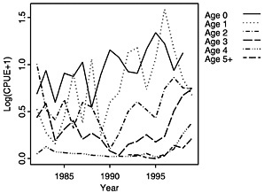
FIGURE D-1b Log(CPUE+1) averaged over surveys for each age class.
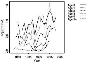
FIGURE D-1c Log(CPUE+1) averaged over surveys for each age class and lagged so that cohort indices coincide.
catch-at-age data as exact and then adapt the resulting range of possible population biomass estimates to fit auxiliary data depicting trends in the biomass. Auxiliary data can include commercial and survey catch rates. The influence of auxiliary data on the estimates is based on a standard goodness-of-fit criterion. The methodology used here is described in detail in Darby and Flatman (1994), and software (Lowestoft Tuning Package) is available to implement it.
The basic idea of the method is that an initial virtual population analysis is conducted from a reasonable but arbitrary starting point to arrive at numbers (N y,a) at year (y) and age (a) for all years and ages:
Ny,a = Ny+1,a+1 eM + Cy,a eM/2.
Here M represents an assumed instantaneous natural mortality rate. Under these values of population size and using observed catch rates ( CPUEf,y,a), estimates of catchability (q) are made for each survey or fleet (f) for each year and age of the analysis:
For each survey-age combination the mean and standard error (SE) of log catchability are calculated across years. Each survey-age mean is then used to produce an estimate of fishing mortality in the most recent year of the survey. This fishing mortality estimate is then prorated up to a survey-based estimate of the fishing mortality generated by all vessels. An inverse variance weighted mean of the various survey results is then calculated. This provides an overall estimate of fishing mortality in the most recent year for each age of fish. Fishing mortality on the oldest age group is set as some specified ratio of the average fishing mortality on some specified range of younger ages. The resulting fishing mortalities for the last year and for the oldest true age in the analysis are then used to reinitiate the VPA.

FIGURE D-2 Log(total catch+1) in thousands by age class.
This cycle continues until the process converges and results stabilize.
The method allows various decisions to be made about the weighting to be applied to past years' data and allows for some weight to be given to an assumption that the fishing mortality in the last year is the same as the average of a specified number of past years. This assumption of “shrinkage” to the mean fishing mortality is most useful when auxiliary tuning data are variable and when not too much trend has occurred in fishing mortality in recent years. The chief virtue of the Laurec-Shepherd method is its simplicity and consequent ease of understanding.
ACON ADAPT
The ADAPT analysis was performed by Robert Mohn of the Canadian Department of Fisheries and Oceans using ACON software.1 The mathematical form of the model closely follows the one described above for the Laurec-Shepherd VPA procedure. The model fits the log of the survey observations at ages 0-4 in the terminal year using a non-linear least-squares algorithm. No “plus group” (i.e., cumulative ages 5 and older) is incorporated. For each year before the terminal year, the fishing mortality (F) at the oldest age (age 4) was estimated as half that of the ages 3, yielding a dome-shaped partial recruitment. Usually, the degree of domedness would be “tuned” by iteration to convergence for recent years; this was not done for this study. The software requires that the observation month for each survey be listed. Because the data were identified by season rather than month, the observation month was approximated by season (e.g., month 7 was assigned to the Northeast Fisheries Science Center summer series). The catchability coefficients (q) for each survey age were determined algebraically at each iteration of the non-linear least-squares algorithm. The error is assumed to be log-normal and the catch is assumed to be error free. Natural mortality was assumed to be 0.2 for all ages and years.

FIGURE D-3 Weight at age in kilograms.
AD Model Builder CAGEAN
The CAGEAN framework differs from the VPA approaches mainly in that it assumes observation variability (ε) associated with the catch data:
Population abundance (N) changes through survivorship, reflecting the combined influences of fishing (F) and natural mortality (M)
Ny+1,a+1 = Ny,a e−(Fy,a+M).
Generally, it is also assumed that fishing mortality can be separated into the product independent year-specific and age-specific components
Fy,a = fysa.
(the so-called separable model assumption). This separable model assumption was relaxed in an effort to explore how it influences interpretations of recruitment. The analysis was conducted using the AD Model Builder software (Fournier, 1996) using a concentrated log-likelihood form for the optimization (Seber and Wild, 1989). Log differences in the sum of squares were applied to the catch and survey observations. Catchability was estimated for each survey data set. A constraint was imposed on the effort deviations reflecting a type of shrinkage assumption as discussed for the VPAs above.
Assessment Results
General Results Across Methods
The three alternative assessment methods were applied independently by different stock assessment scientists to the same summer flounder data and compared with the NMFS 1999 assessment results. The general trends in spawning stock biomass (Figure D-4) and fishing mortality (Figure D-5) averaged over ages 2 through 4 appear similar although there is not an exact correspondence. There appears to have been a general decline in the stock from 1982 through 1990, followed by a general increase in stock biomass through the 1990s. Complementary trends can be seen in the corresponding fishing mortality estimates, with an increase shown in the 1980s and a decrease in the 1990s.
Two things are worth noting in viewing these trends. First, the range of estimates varies substantially under the different model formulations, indicating that even with the same data, different models, employing different assumptions and implemented by different scientists, can produce different results. Second, the biomass trends in the last three years differ among methods, with certain estimates going in opposite directions. Although this is certainly problematic for managers and stakeholders who are trying to make management decisions, it must be recognized that the variability among models in the last years is greater than the inter-annual variability of any specific model. Nonetheless, departures in the relative trends in abundance between models indicates that we should further explore how the models respond to the data.
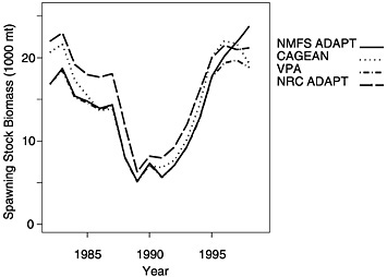
FIGURE D-4 Summer flounder spawning stock biomass as estimated by NMFS, as compared with three independently conducted model applications.
NOTE: NMFS = National Marine Fisheries Service; NRC = National Research Council; and VPA = virtual population analysis. ADAPT and CAGEAN are two stock assessment techniques, as described in the text.

FIGURE D-5 Summer flounder fishing mortality for ages 2-4 as estimated by NMFS and compared with three independently conducted model applications.
Laurec-Shepherd VPA
Figure D-6 shows graphs of the residuals of Ln(q[f,y,a]) for each survey, with different symbols to show the ages. A number of points become apparent from these graphs.
-
Most series are quite variable. Residuals of greater than 1 (and less than −1) are common.
-
A number of the series may have some auto-correlation with long-term variations between higher and lower catchability.
-
These trends often seem similar between the various age classes represented by different surveys, but the trends vary among surveys. This might suggest variation in local availability to the various (mostly area-based) surveys rather than some change (e.g., mis-reporting errors on catchat-age data) that would be reflected in all series.
The standard errors of the Ln(q[f,y,a]) calculated from the full 1998 SAW tuning data are shown in Table D-2. These include an input value of 0.5 for the shrinkage mean. In general the standard errors are quite high. Most are higher than 0.5, which corresponds approximately to a 50% coefficient of variation.
The standard errors in Table D-2 may be converted to the inverse variances used to combine estimates of fishing mortality in the last year (1998) of the analysis (results are shown in Table D-3). It is apparent that the Laurec-Shepherd method gives substantially more weight to the results for some surveys for some ages than others (e.g., on age 0, the New Jersey survey gets an 18 percent weighting, whereas Rhode Island fixed station survey gets only 3 percent). The Delaware 30-foot Trawl Survey gets a low weighting for young fish but a higher weighting for 2-and 3-year-old fish. The shrinkage mean for each of the 4 ages gets a weighting of about 13 to 16 percent.
The combined estimates of standard error of the terminal fishing mortality on ages 0-3 are 0.22, 0.27, 0.22, and 0.20, respectively. Thus, considerable variation might be expected in the various estimates of fishing mortality rate and population size at age.
A further diagnostic given by the Lowestoft

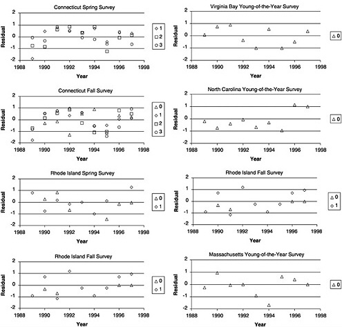
FIGURE D-6 Plots of the residuals of the natural log of catchability (Ln[Q]) of each survey from Laurec-Shepherd tuning of summer flounder data.
software package is the slope and standard error of the slope of a regression of q(f,y,a) on y for each survey and age. Table D-4 shows the ratios of slope to its standard error for each available combination of survey and age. Depending on degrees of freedom, only levels of this ratio over 2 might be regarded as being significant. As might be expected from groundfish surveys, only a few of the series reach this level: only NEFSC winter survey for ages 2 and 3, the NEFSC autumn survey for age 1, and the Rhode Island fixed station survey for age 0. The significance of the NEFSC winter survey probably results because it is a short time-series with only the downswing of a cycle included. It would therefore seem inappropriate to adjust this series for linear trends in catchability.
TABLE D-2 Standard Errors of the Natural Log-transformed Survey Catchability
|
Age |
||||
|
Survey |
0 |
1 |
2 |
3 |
|
NEFSC Spring Survey |
0.555 |
0.52 |
0.616 |
|
|
NEFSC Winter Survey |
0.625 |
0.82 |
0.569 |
|
|
NEFSC Fall Survey |
0.735 |
0.468 |
0.719 |
0.609 |
|
Massachusetts Spring Survey |
1.024 |
0.82 |
0.655 |
|
|
Massachusetts Fall Survey |
1.187 |
0.521 |
0.617 |
|
|
Connecticut Spring Survey |
0.866 |
0.639 |
0.507 |
|
|
Connecticut Fall Survey |
0.707 |
0.607 |
0.628 |
0.707 |
|
Rhode Island Spring Survey |
0.921 |
1.015 |
||
|
Rhode Island Fall Survey |
0.784 |
0.796 |
||
|
Rhode Island Fixed Station Survey |
0.97 |
0.707 |
||
|
New Jersey Survey |
0.427 |
0.626 |
0.834 |
1.131 |
|
Delaware 16-foot Trawl Survey |
0.815 |
|||
|
Delaware 30-foot Trawl Survey |
1.465 |
1.059 |
0.616 |
0.479 |
|
Virginia Rivers Young-of-the-Year Survey |
0.532 |
|||
|
Virginia Bay Young-of-the-Year Survey |
0.664 |
|||
|
North Carolina Young-of-the-Year Survey |
0.732 |
|||
|
Maryland Young-of-the-Year Survey |
0.599 |
|||
|
Massachusetts Young-of-the-Year Survey |
0.9 |
|||
|
Shrinkage Mean |
0.5 |
0.5 |
0.5 |
0.5 |
TABLE D-3 Weightings Applied to Each Age of Each Survey (percentages)
|
Age |
||||
|
Survey |
0 |
1 |
2 |
3 |
|
NEFSC Spring Survey |
0% |
12% |
15% |
9% |
|
NEFSC Winter Survey |
0% |
9% |
6% |
11% |
|
NEFSC Fall Survey |
6% |
16% |
8% |
9% |
|
Massachusetts Spring Survey |
0% |
3% |
6% |
8% |
|
Massachusetts Fall Survey |
0% |
3% |
15% |
9% |
|
Connecticut Spring Survey |
0% |
5% |
10% |
14% |
|
Connecticut Fall Survey |
6% |
10% |
10% |
7% |
|
Rhode Island Spring Survey |
4% |
3% |
0% |
0% |
|
Rhode Island Fall Survey |
5% |
6% |
0% |
0% |
|
Rhode Island Fixed Station Survey |
3% |
7% |
0% |
0% |
|
New Jersey Survey |
18% |
9% |
6% |
3% |
|
Delaware 16-foot Trawl Survey |
5% |
0% |
0% |
0% |
|
Delaware 30-foot Trawl Survey |
2% |
3% |
10% |
15% |
|
Virginia Rivers Young-of-the-Year Survey |
11% |
0% |
0% |
0% |
|
Virginia Bay Young-of-the-Year Survey |
7% |
0% |
0% |
0% |
|
North Carolina Young-of-the-Year Survey |
6% |
0% |
0% |
0% |
|
Maryland Young-of-the-Year Survey |
9% |
0% |
0% |
0% |
|
Massachusetts Young-of-the-Year Survey |
4% |
0% |
0% |
0% |
|
Shrinkage Mean |
13% |
14% |
16% |
14% |
TABLE D-4 Slope of the Regression of Catchability for Each Survey, Year, and Age (q[f,y,a]) Divided by the Standard Error of the Slope
|
Age |
||||
|
Survey |
0 |
1 |
2 |
3 |
|
NEFSC Spring Survey |
0.44 |
−0.83 |
−1.37 |
|
|
NEFSC Winter Survey |
−1.35 |
−6.13 |
−2.34 |
|
|
NEFSC Fall Survey |
1.29 |
3.02 |
1.72 |
−0.46 |
|
Massachusetts Spring Survey |
0.17 |
0.82 |
0.14 |
|
|
Massachusetts Fall Survey |
−0.49 |
−0.75 |
0.73 |
|
|
Connecticut Spring Survey |
0.47 |
0.99 |
0.55 |
|
|
Connecticut Fall Survey |
−0.40 |
−0.04 |
0.76 |
−0.14 |
|
Rhode Island Spring Survey |
−1.31 |
−0.15 |
||
|
Rhode Island Fall Survey |
−0.55 |
−0.58 |
||
|
Rhode Island Fixed Station Survey |
3.33 |
1.50 |
||
|
New Jersey Survey |
1.66 |
1.41 |
0.77 |
1.31 |
|
Delaware 16-foot Trawl Survey |
0.01 |
|||
|
Delaware 30-foot Trawl Survey |
−0.88 |
−1.27 |
−0.16 |
−1.31 |
|
Virginia Rivers Young-of-the-Year Survey |
−1.23 |
|||
|
Virginia Bay Young-of-the-Year Survey |
−0.42 |
|||
|
North Carolina Young-of-the-Year Survey |
1.90 |
|||
|
Maryland Young-of-the-Year Survey |
1.65 |
|||
|
Massachusetts Young-of-the-Year Survey |
1.50 |
|||
The Lowestoft package allows the Laurec-Shepherd method to be run in retrospective mode (Box D-1). This shows the interpretation that the method would have placed on the current data set if the components that would have been available in past years were used to tune the VPA in those years. It thus gives some feel for the variability of the results and also can indicate biases in the analysis. Figure D-7, Figure D-8, Figure D-9 and Figure D-10 show the retrospective patterns of estimates of fishing mortality rate, spawning stock biomass, total stock biomass, and recruitment at age 0 for summer flounder. The figures indicate that past interpretations might have differed by as much as double or half from more recent and presumably better estimates of the value of fishing mortality (e.g., 1992 or 1994). In recent years the results seem more consistent, as shown by more convergence among the lines that extend to later years. These results translate into somewhat reduced and opposite retrospective patterns in SSB and total stock biomass. This is in contrast to the NMFS results, which show little variation in SSB. The weightings calculated for each survey and age group in each year of the retrospective analysis are given in Table D-5.
Since the fishing mortality decreased in recent years, the advisability of using shrinkage to the mean needs to be questioned. Consequently, a fresh set of retrospective results were generated using the Laurec-Shepherd method on the 1998 tuning set for summer flounder without applying shrinkage to the mean (not shown). On the whole, these results seem more variable than those obtained using the shrinkage option, indicating that
the variability seen in the data may be interpreted as observation error, bias, or a systematic trend in the underlying process (e.g., in fish catchability). Identification of the underlying process will improve predictions as the appropriate level of variation will be better represented.
|
BOX D-1 Retrospective Analysis in Stock Assessments (NRC, 1998a) The reliance of most stock assessment models on time-series data implies not only that each successive assessment characterizes current stock status and other parameters used for management, but also that the complete time series of past abundance estimates is updated. Retrospective analysis is the examination of the consistency among successive estimates of the same parameters obtained as new data are gathered. Either the actual results from historical assessments are used or, to isolate the effects of changes in methodology, the same method is applied repeatedly to segments of the data series to reproduce what would have been obtained annually if the newest method had been used for past assessments. Retrospective analysis has been applied most commonly to age-structured assessments (Sinclair et al., 1991; Mohn, 1993; Parma, 1993; Anon., 1995). In such applications, the statistical variance of the abundance (or fishing mortality) estimates tends to decrease with time elapsed; estimates of the last year (those used for setting regulations) are the least reliable. In retrospective analysis, abundance estimates for the final years of each data series can vary substantially among successive updates, whereas those for the early years tend to converge to stable values. In some cases (i.e., some northwest Atlantic cod stocks, Pacific halibut, North Sea sole), early abundance estimates are consistently biased (either upward or downward) with respect to corresponding estimates obtained in later assessments. Extreme cases of consistent overestimation of stock abundance can have disastrous management consequences, as illustrated by the collapse of the Newfoundland northern cod (Hutchings and Myers, 1994; Walters and Pearse, 1996). Retrospective biases can arise for many reasons, ranging from bias in the data (e.g., catch misreporting) to different types of model misspecification (mostly parameters that are assumed to be constant in the analysis but actually change, as well as incorrect assumptions about relative vulnerability of age classes). In traditional retrospective analyses, successive assessments use data for different periods, all starting at the same time with one year of data added to each assessment. An alternative method is to conduct successive assessments using data for a moving window of a fixed number of years (as in Parma, 1993, and Deriso et al., 1985). This method is appropriate for exploring trends in parameter estimates. |
ACON ADAPT
The summary statistics from the fit of log numbers at age for the 5 terminal ages are:
|
Age |
Param |
CV |
Bias (percent) |
|
0 |
9.88058 |
0.336 |
−0.0121 |
|
1 |
9.61357 |
0.281 |
0.0263 |
|
2 |
9.10554 |
0.272 |
0.0859 |
|
3 |
8.687 |
0.283 |
0.0981 |
|
4 |
6.63158 |
0.435 |
0.5283 |
The residuals (log[prediction/observation]) from the fit and the mean square error for each survey-age are given in Figure D-11. These patterns often have diagnostic value, which is
FIGURE D-7 Retrospective estimates of fishing mortality (F) for summer flounder using the full 1998 data set (with shrinkage to past F).
FIGURE D-8 Retrospective estimates of spawning stock biomass (SSB) for summer flounder using the full 1998 data set (with shrinkage to past F).
somewhat confused in the present instance because of the relatively large number of indices. Vertical patterns suggest a year effect, for example, the terminal year of the NEFSC.w survey has large positive residuals for all ages. Indices with large mean square residuals may be removed. Also, a correlation analysis may be done among the residuals to identify redundant or contradictory series.
FIGURE D-9 Retrospective estimates of total stock biomass (TSB) for summer flounder using the full 1998 data set (with shrinkage to past F).
FIGURE D-10 Retrospective estimates of recruitment (at notional age 0) in millions (recruits in thousands) for summer flounder using the full 1998 data set (with shrinkage to past F).
The fitted numbers for each survey and the data, after scaling for the catchabilities, are shown in Figure D-12. Figure D-13 summarizes the results of the sequential population analysis. The upper plot is the spawning stock biomass aged ahead (mortality applied) to August. The lower plot is the average (unweighted) F for ages 1-3.
A retrospective analysis was performed using average F over ages 1-3 and August biomass
TABLE D-5 Weights Applied for Each Year of Retrospective Analysis
|
1988 |
1989 |
1990 |
1991 |
1992 |
1993 |
1994 |
1995 |
1996 |
1997 |
1998 |
|
|
Northeast Fisheries Science Center Spring Survey |
|||||||||||
|
0 |
0 |
0 |
0 |
0 |
0 |
0 |
0 |
0 |
0 |
0 |
0 |
|
1 |
0.0687 |
0.0624 |
0.0592 |
0.0636 |
0.0504 |
0.0683 |
0.072 |
0.0739 |
0.0726 |
0.0782 |
0.1156 |
|
2 |
0.0369 |
0.1048 |
0.1207 |
0.0796 |
0.0768 |
0.0935 |
0.0971 |
0.1221 |
0.113 |
0.1367 |
0.1459 |
|
3 |
0.0692 |
0.0674 |
0.0696 |
0.0684 |
0.0523 |
0.0812 |
0.0885 |
0.0973 |
0.0556 |
0.071 |
0.0928 |
|
Northeast Fisheries Science Center Winter Survey |
|||||||||||
|
0 |
0 |
0 |
0 |
0 |
0 |
0 |
0 |
0 |
0 |
0 |
0 |
|
1 |
0 |
0 |
0 |
0 |
0 |
0 |
0 |
0 |
0.0945 |
0.075 |
0.0912 |
|
2 |
0 |
0 |
0 |
0 |
0 |
0 |
0 |
0 |
0.1951 |
0.0882 |
0.0587 |
|
3 |
0 |
0 |
0 |
0 |
0 |
0 |
0 |
0 |
0.077 |
0.0792 |
0.1087 |
|
Northeast Fisheries Science Center Fall Survey |
|||||||||||
|
0 |
0.1199 |
0.1477 |
0.1381 |
0.0889 |
0.0457 |
0.0555 |
0.0512 |
0.0472 |
0.0624 |
0.0621 |
|
|
0.06 |
|||||||||||
|
1 |
0.3614 |
0.5409 |
0.5504 |
0.5628 |
0.4426 |
0.3331 |
0.3119 |
0.2991 |
0.3145 |
0.3264 |
0.1626 |
|
2 |
0.038 |
0.1406 |
0.1602 |
0.1319 |
0.1243 |
0.0911 |
0.1184 |
0.1008 |
0.0907 |
0.0934 |
0.0763 |
|
3 |
0.2244 |
0.2216 |
0.23 |
0.2237 |
0.2473 |
0.2109 |
0.1959 |
0.1482 |
0.0809 |
0.0862 |
0.0949 |
|
Massachusetts Department of Marine Fisheries Spring Survey |
|||||||||||
|
0 |
0 |
0 |
0 |
0 |
0 |
0 |
0 |
0 |
0 |
0 |
0 |
|
1 |
0.0375 |
0.031 |
0.033 |
0.0277 |
0.0246 |
0.0412 |
0.0283 |
0.0274 |
0.0226 |
0.0251 |
0.034 |
|
2 |
0.0112 |
0.0314 |
0.0449 |
0.0274 |
0.0264 |
0.038 |
0.0366 |
0.038 |
0.0394 |
0.0514 |
0.0587 |
|
3 |
0.0405 |
0.0433 |
0.048 |
0.0446 |
0.0505 |
0.0564 |
0.0609 |
0.0685 |
0.0485 |
0.0653 |
0.082 |
|
Massachusetts Department of Marine Fisheries Fall Survey |
|||||||||||
|
0 |
0 |
0 |
0 |
||||||||
|
1 |
0.0216 |
0.0172 |
0.0196 |
0.0225 |
0.0178 |
0.0267 |
0.0241 |
0.0258 |
0.0262 |
0.033 |
0.0253 |
|
2 |
0.0222 |
0.082 |
0.133 |
0.1386 |
0.0908 |
0.1999 |
0.1604 |
0.1405 |
0.1099 |
0.1318 |
0.1453 |
|
3 |
0.053 |
0.0601 |
0.0627 |
0.0726 |
0.0763 |
0.0978 |
0.1004 |
0.1187 |
0.0668 |
0.0795 |
0.0925 |
|
Connecticut Department of Environmental Protection Spring Survey |
|||||||||||
|
0 |
0 |
0 |
0 |
0 |
0 |
0 |
0 |
0 |
0 |
0 |
0 |
|
1 |
0.0188 |
0.017 |
0.018 |
0.0203 |
0.0171 |
0.0268 |
0.0276 |
0.0291 |
0.0281 |
0.0343 |
0.0475 |
|
2 |
0.0525 |
0.1358 |
0.1942 |
0.1347 |
0.105 |
0.0949 |
0.075 |
0.088 |
0.0786 |
0.0923 |
0.0966 |
|
3 |
0.1624 |
0.1934 |
0.214 |
0.2199 |
0.1966 |
0.189 |
0.1862 |
0.2259 |
0.1163 |
0.1368 |
0.1369 |
|
Connecticut Department of Environmental Protection Fall Survey |
|||||||||||
|
0 |
0 |
0 |
0.0889 |
0.0939 |
0.0392 |
0.0454 |
0.0611 |
0.0542 |
0.0569 |
0.0674 |
0.0648 |
|
1 |
0.1574 |
0.054 |
0.0537 |
0.0541 |
0.0444 |
0.0663 |
0.067 |
0.0668 |
0.0597 |
0.0683 |
0.0967 |
|
2 |
0.792 |
0.3854 |
0.1651 |
0.3176 |
0.2123 |
0.1646 |
0.1884 |
0.1538 |
0.0919 |
0.0966 |
0.1 |
|
3 |
0.2244 |
0.2076 |
0.1801 |
0.1733 |
0.1565 |
0.1252 |
0.1351 |
0.1207 |
0.057 |
0.0624 |
0.0704 |
|
Rhode Island Department of Fish and Wildlife Spring Survey |
|||||||||||
|
0 |
0.0211 |
0.019 |
0.022 |
0.0222 |
0.0155 |
0.0182 |
0.0196 |
0.0216 |
0.0264 |
0.0325 |
0.0382 |
|
1 |
0.0308 |
0.0265 |
0.0283 |
0.0332 |
0.0269 |
0.0439 |
0.0475 |
0.0485 |
0.0279 |
0.0282 |
0.0346 |
|
2 |
0 |
0 |
0 |
0 |
0 |
0 |
0 |
0 |
0 |
0 |
0 |
|
3 |
0 |
0 |
0 |
0 |
0 |
0 |
0 |
0 |
0 |
0 |
0 |
|
Rhode Island Department of Fish and Wildlife Fall Survey |
|||||||||||
|
0 |
0.0359 |
0.0324 |
0.0333 |
0.0308 |
0.018 |
0.025 |
0.0257 |
0.028 |
0.0401 |
0.0458 |
0.0527 |
|
1 |
0.0816 |
0.0665 |
0.0664 |
0.0455 |
0.039 |
0.0582 |
0.0611 |
0.0597 |
0.0494 |
0.0503 |
0.0562 |
|
2 |
0 |
0 |
0 |
0 |
0 |
0 |
0 |
0 |
0 |
0 |
0 |
|
3 |
0 |
0 |
0 |
0 |
0 |
0 |
0 |
0 |
0 |
0 |
0 |
|
Rhode Island Department of Fish and Wildlife Fixed-station Survey |
|||||||||||
|
0 |
0 |
0 |
0 |
0 |
0 |
0 |
0 |
0 |
0.0283 |
0.0338 |
0.0344 |
|
1 |
0 |
0 |
0 |
0 |
0 |
0 |
0.0884 |
0.0813 |
0.0585 |
0.0518 |
0.0713 |
|
2 |
0 |
0 |
0 |
0 |
0 |
0 |
0 |
0 |
0 |
0 |
0 |
|
3 |
0 |
0 |
0 |
0 |
0 |
0 |
0 |
0 |
0 |
0 |
0 |
|
New Jersey Department of Fish and Wildlife Survey |
|||||||||||
|
0 |
0 |
0 |
0 |
0 |
0.2307 |
0.0739 |
0.1222 |
0.079 |
0.1536 |
0.1417 |
0.1777 |
|
1 |
0 |
0 |
0 |
0 |
0.2136 |
0.158 |
0.1014 |
0.1101 |
0.0969 |
0.0882 |
0.0909 |
|
2 |
0 |
0 |
0 |
0 |
0.2345 |
0.1479 |
0.1349 |
0.1058 |
0.0604 |
0.0531 |
0.0567 |
|
3 |
0 |
0 |
0 |
0 |
0.0324 |
0.031 |
0.034 |
0.0327 |
0.0217 |
0.0239 |
0.0275 |
|
Delaware Department of Fish and Wildlife 16-Foot Trawl Survey |
|||||||||||
|
0 |
0.1819 |
0.1225 |
0.0987 |
0.0823 |
0.0351 |
0.0439 |
0.0363 |
0.0357 |
0.0465 |
0.046 |
0.0488 |
|
1 |
0 |
0 |
0 |
0 |
0 |
0 |
0 |
0 |
0 |
0 |
0 |
|
2 |
0 |
0 |
0 |
0 |
0 |
0 |
0 |
0 |
0 |
0 |
0 |
|
3 |
0 |
0 |
0 |
0 |
0 |
0 |
0 |
0 |
0 |
0 |
0 |
|
Delaware Department of Fish and Wildlife 30-Foot Trawl Survey |
|||||||||||
|
0 |
0 |
0 |
0 |
0 |
0 |
0 |
0 |
0.0112 |
0.0164 |
0.014 |
0.0151 |
|
1 |
0 |
0 |
0 |
0 |
0 |
0 |
0 |
0.0301 |
0.0297 |
0.022 |
0.0318 |
|
2 |
0 |
0 |
0 |
0 |
0 |
0 |
0 |
0.0715 |
0.0749 |
0.0951 |
0.104 |
|
3 |
0 |
0 |
0 |
0 |
0 |
0 |
0 |
0 |
0.3614 |
0.2607 |
0.1534 |
|
Virginia Rivers Young-of-the-Year Survey |
|||||||||||
|
0 |
0.126 |
0.1787 |
0.1649 |
0.1421 |
0.0779 |
0.0815 |
0.0899 |
0.0989 |
0.1099 |
0.1106 |
0.1145 |
|
Virginia Institute of Marine Sciences Survey, including Chesapeake Bay Young-of-the-Year |
|||||||||||
|
0 |
0 |
0 |
0 |
0 |
0.2 |
0.0786 |
0.083 |
0.0723 |
0.0736 |
0.0717 |
0.0735 |
|
North Carolina Young-of-the-Year Survey |
|||||||||||
|
0 |
0 |
0 |
0 |
0.1599 |
0.1042 |
0.281 |
0.2438 |
0.2946 |
0.0692 |
0.0666 |
0.0605 |
|
Maryland Young-of-the-Year Survey |
|||||||||||
|
0 |
0.1267 |
0.1185 |
0.1125 |
0.1019 |
0.0714 |
0.1029 |
0.0926 |
0.0849 |
0.1238 |
0.1164 |
0.0903 |
|
Massachusetts Young-of-the-Year Survey |
|||||||||||
|
0 |
0.0715 |
0.0792 |
0.0748 |
0.0671 |
0.0392 |
0.0508 |
0.0403 |
0.0402 |
0.0489 |
0.0536 |
0.04 |
|
Shrinkage Mean |
|||||||||||
|
0 |
0.317 |
0.302 |
0.2668 |
0.2108 |
0.1229 |
0.1432 |
0.1342 |
0.1322 |
0.1439 |
0.1378 |
0.1296 |
|
1 |
0.2221 |
0.1845 |
0.1714 |
0.1703 |
0.1234 |
0.1775 |
0.1708 |
0.1482 |
0.1194 |
0.1191 |
0.1425 |
|
2 |
0.0472 |
0.12 |
0.182 |
0.1702 |
0.1298 |
0.17 |
0.1892 |
0.1794 |
0.1463 |
0.1613 |
0.1578 |
|
3 |
0.2262 |
0.2067 |
0.1956 |
0.1976 |
0.188 |
0.2084 |
0.1991 |
0.1879 |
0.1149 |
0.1351 |
0.1408 |

FIGURE D-11 Expanded symbol diagram of residuals of abundance measures from sequential population analysis. Circles and crosses represent negative and positive residuals respectively, with the size of the symbol being proportional to the size of the residual. The left-hand column denotes the survey and ages while the right-hand column shows the mean square residual (MSR) for each survey-age.
NOTE: CTDEP = Connecticut Department of Environmental Protection; CTYOY = Connecticut Young-of-the-Year Survey; MADMF = Massachusetts Department of Marine Fisheries; MDYOY = Maryland Young-of-the-Year Survey; NCYOY = North Carolina Young-of-the-Year Survey; NEFSC = Northeast Fisheries Science Center; NEYOY = New England Young-of-the-Year Survey; NJBMF = New Jersey Bureau of Marine Fisheries; NJYOY = New Jersey Young-of-the-Year Survey; RIDFW = Rhode Island Department of Fish and Wildlife; VAYOY = Virginia Young-of-the-Year Survey, f = fall survey; s = spring survey; w = winter survey.
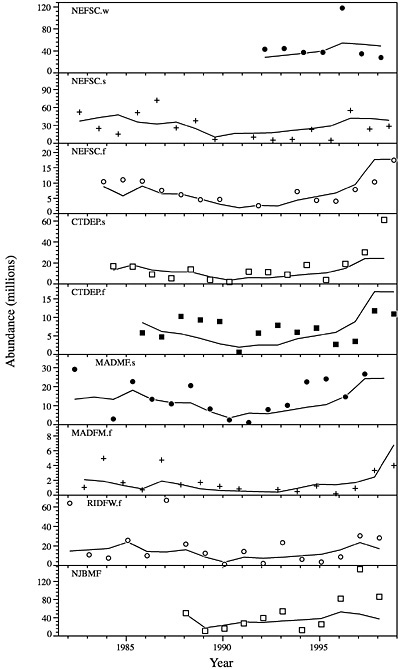
FIGURE D-12 Predicted population size and data from each survey. The data are summed over the appropriate ages, which are shown in Figure D-11.

FIGURE D-13 Sequential population analysis (SPA) estimates of F and biomass from ADAPT base run using data shown in Figure D-1. The biomass has been aged ahead to August and weighted by a maturity ogive (a continuous cumulative frequency curve).
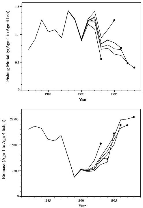
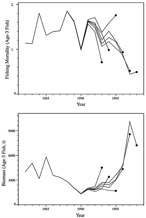

FIGURE D-16 Relative retrospective patterns for F and biomass at age 3. The estimates in Figure D-15 have been divided by the longest time series to obtain the values shown above.
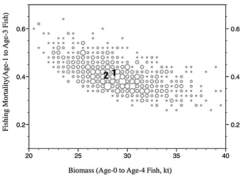
FIGURE D-17 Expanded symbol diagram of terminal F and biomass from 1,000 bootstrap trials. “1” marks the point estimate and “2” marks the bias-corrected estimate.
over ages 1-4 (see Figure D-14). The retrospective pattern for the Fs seems worse than that for the biomass, in that the former diverge more substantially. The apparent discrepancy was analyzed further. The first effect removed was the different weighting implied when F values are averaged but biomass values are summed. This was done by looking at the patterns for age 3 alone (see Figure D-15). Here, the F still has more scatter of the terminal points of retrospective curves. Figure D-16 recasts Figure D-15 as relative retrospective patterns. Each line in Figure D-15 was scaled relative to the longest series. Here the two patterns look similar, though inverted. This demonstration showed that the apparent discrepancy was due to the different weighting and the non-linear relationship between F and numbers at age and not an error in computation.
The performance of the model was further tested by a bootstrap analysis. The residuals from the base run were re-sampled to produce 1,000 bootstrapped replicate surveys. The catch data were then fit to the replicates. The terminal average F and biomass were aggregated and plotted in Figure D-17. The cloud of symbols is well behaved in the sense that it forms a continuous mass. In some instances, this type of analysis will reveal separate clouds, which can reflect instability in the analysis. The number “1” denotes the point estimate and the number “2” is the bias-corrected estimate. The bias is estimated by taking the difference between the point estimate and the mean of the bootstrap estimates, which is then
applied to the point estimate to produce the biascorrected values.
FIGURE D-18 Comparisons of CAGEAN AD Model Builder results with varying selectivity at age (with error bars) and NMFS ADAPT results (same as in Figure D-4).
The analysis of summer flounder has more surveys than are usually included, and was performed in some haste. Although we consider this ADAPT analysis of the summer flounder data to be preliminary, we believe that the results are useful for NMFS as a basis for a more complete evaluation of their ADAPT approach. If a more complete investigation and comparison with other analyses were deemed desirable, considerable time should be set aside by NMFS for such an exercise, which would help quality control.
AD Model Builder CAGEAN
The most significant difference between the conventional CAGEAN-type analysis and the conventional VPA approach in terms of the summer flounder assessment is the assumption of separability between the year and age effects included in the CAGEAN procedure. This separability assumption carries with it the implication of a constant selectivity at age over time as employed here. Changes observed in this fishery might cause selectivity to vary with changes in regulations (e.g., mesh size), making an assumption of constant selectivity inappropriate. To address this issue a modification was made to the CAGEAN model to allow for some variation in selectivity with time. This was done by allowing deviations to occur in the log selectivity at age with a penalty applied to the sum of the squared deviations in the log-likelihood formulation used to specify the optimization surface. It was only when deviations were allowed for age classes 0 and 1 that any substantial change in the estimates result. When the CAGEAN model was used with varying selectivity at age 0 and age 1, the spawning stock biomass estimates more closely follow that derived under the 1999 NMFS assessment (Figure D-18). Selectivity estimates, as portrayed in fishing mortality estimates at age shown in Figure D-19, show a sharp drop in recent years, which the model assumes corresponds to changes in gear and targeting practices in the commercial and recreational fisheries. If such an assumption
is erroneous, other factors, such as a drop in recruitment, could explain the trends.
FIGURE D-19 Estimates of fishing mortality from CAGEAN model with varying selectivity at age.
The influence of this change in selectivity under this model formulation is similar and perhaps analogous to responses in model estimates to the shrinkage assumption in F employed by the other assessment methods. All these results point to the rather tenuous nature of the estimates available for the most recent years.
SUMMARY
Three analyses of summer flounder data by three different individuals using three different stock assessment models yielded the same general decadal trends indicated by the 1999 National Marine Fisheries Service assessment (see Figure D-4 and Figure D-5). Namely, these analyses showed that the spawning stock biomass has recovered substantially from a trough in the early 1990s and that fishing mortality dropped substantially during the same period. The committee believes both changes are probably due to strict management measures implemented in 1992.
However, the models yielded some differences in estimates. Because all the models used the same data, differences in the estimates arose from differences in the structural assumptions of each modeling method. Model structure introduces implicit assumptions, and some models are built to be easier to use by specifying assumptions in the standard computer software rather than allowing stock assessment scientists to vary the assumptions through input values. These assumptions often go unstated, but in this case conflicting signals in the data dramatically influenced model results because of the assumptions used. Our analysis does not necessarily indicate that the NMFS results are incorrect or that any of our specific results are correct. However, the analysis does show that the assumptions are influencing the results and that their influence should be acknowledged explicitly and used to help understand the dynamics of fish populations.
The committee was able to narrow the likely causes of these differences and believes they are related to the structure imposed on fishing mortality at age in the various models. This structure
is implemented in the assumption of separable selectivity and full recruitment fishing mortality in the CAGEAN model and by the level set for the “shrinkage” control assumption in the VPA and ADAPT models. The separable selectivity assumption in the CAGEAN model forces selectivity at age to remain fixed over time. The shrinkage factor, used in the ADAPT and VPA models, controls how quickly fishing mortality (F) is allowed to change from year to year.
The CAGEAN model shows the most distinct drop in spawning stock biomass in recent years because it does not have the flexibility to deal with the decrease in younger fish seen in both CPUE and catch-at-age data. The behaviors of the VPA and ADAPT models appear to be related to the degree of variability in fishing mortality allowed through the shrinkage applied to fishing mortality at age. Although the controls imposed by these models take place through different mechanisms, both types of controls decrease the degree to which the estimates of fishing mortality at age can depart from what was estimated in the past. We believe that some degree of shrinkage is appropriate in all assessment models, because if the F values are not constrained they may drift, especially for younger age classes in the most recent years. Alternatively, if analysts believe that F values should not be constrained, the analysts should justify why fishing mortality at age for these younger age classes is expected to change (e.g., through changes in recruitment or in the bycatch or discard mortality rates). Such changes may not be obvious in outputs showing only annual fishing mortalities averaged over age classes.
Models differ in how they deal with conflicting data, such as seen in the survey CPUE data (Figure D-1c). The relative abundance indices may have peaked with the 1995 cohort. The trends indicated by the two observations available for the 1998 cohort (shown in Figure D-1c as age 0 and age 1) go in opposite directions; the survey CPUE of year-0 summer flounder is increasing, whereas the survey CPUE for year-1 fish is decreasing. This creates a conflict in the data that may lead to equally likely, but conflicting, trends in model estimates. To explore and address this issue, a modification was made to the CAGEAN model to allow for some variation in selectivity over time. 2 When the CAGEAN model was used with varying selectivity at age 0 and age 1, the spawning stock biomass estimates more closely followed those derived under the 1999 NMFS assessment (Figure D-18). This indicates that the selectivity assumption caused at least some of the differences in the outputs of the NMFS ADAPT and CAGEAN models. Selectivity estimates, as portrayed in fishing mortality estimates at age (shown in Figure D-19), show a sharp drop in recent years, which the model assumes corresponds to changes in selectivities in commercial and recreational fisheries. This assumption, if false, could mask more serious alternative processes that also could provide an explanation for the trends, such as a drop in recruitment in recent years.
Estimated fishing mortality rates varied greatly among the models (Figure D-5). In the last year of the series, each method produced almost the same estimate of fishing mortality, yet all are above the fisheries management target level for F of 0.24.
Stock assessment scientists responsible for summer flounder should investigate how differences among model results arise and whether such differences indicate changes needed in the models or assumptions used. NMFS should try to test the effects of shrinkage and should investigate the conflicting trends in the youngest year classes. As stated in the 1998 NRC report Improving Fish Stock Assessments (NRC, 1998a):
Because there are often problems with the data used in assessments, a variety of different assessment models should be applied to the same data. The different views pro-
|
2 |
This was done by allowing deviations to occur in the log selectivity-at-age with a penalty applied to the sum of the squared deviations in the log-likelihood formulation used to specify the optimization surface. |
vided by different models should improve the quality of assessment results. (p. 113)
This advice is borne out by the current committee's reassessment of summer flounder data.
In the summer flounder case, the NMFS assessment could be improved by analyzing the same data using different models. The differences obtained should help analysts learn about problems in the data, problems in using the ADAPT model with these data, or problems with the assumptions used in the NMFS ADAPT model (e.g., related to shrinkage and changes in selectivity over time).


