Innovations to Locate Stacked or Deep Utilities (2014)

Below is the uncorrected machine-read text of this chapter, intended to provide our own search engines and external engines with highly rich, chapter-representative searchable text of each book. Because it is UNCORRECTED material, please consider the following text as a useful but insufficient proxy for the authoritative book pages.

32 Combined Technical Assessment of SHRP 2 Projects R01B and R01C Executive Summary The objective of this project is to design, construct, and test prototype instruments for locating buried utilities. These pro- totypes will be based on new and emerging technologies. The first step is the review of existing and promising technologies for location and tracing of buried infrastructure as applied to deeply buried pipe. This review is intended to ensure that this project does not repeat previous efforts, to verify the need for new location tools, to define operating needs of the industry, to provide the stakeholders information to accurately assess emerging technologies, and to provide confidence that the proposed methods can succeed. A number of comprehensive technology reviews have recently been completed (1, 2, 3). These reviews cover existing, emerging, and conceptual ideas for utility location technolo- gies. SHRP 2 Report S2-R01-RW is especially comprehensive, reviewing the literature with more than 350 references (1). SHRP 2 R01A also reviewed locating technology. The Gas Technology Institute (GTI) performed a study for a number of natural-gas utilities that tested commercially available pipe location techniques (4). Part of that study also evalu- ated emerging technology. All the studies identify the same technologies that are promising but require near-term devel- opment. One conclusion reached in all the studies is that no single tool can function well in all soil conditions. For exam- ple, ground-penetrating radar (GPR) is good in dry, non- conducting soil, but it cannot detect utilities more than 3 to 4 ft deep in wet clay. Therefore a range of complementary techniques is required. These could be combined into a single system or applied as individual tools. The ability to assess the new technologies and understand how they complement each other requires understanding soil properties and wave propagation. This appendix summarizes the key electromagnetic and acoustic wave properties and soil properties with the goal of providing understanding of why various technologies function well in some soils and not in others. This information permits assessment of technologies in terms of the ultimate depth location. Next, the operating principles behind the commercially available and most prom- ising technologies are described, including their strengths and weaknesses. A brief description of how the new tech- nologies will improve deep utility location is given. Analysis of this information justifies development of seis- mic, active acoustic, smart tag, inertial guidance system, and electromagnetic (EM) technologies as applied to deeply buried utilities. Introduction This appendix reviews existing and promising technologies for location and tracing of buried infrastructure as applied to bur- ied utilities. Ideally, a tool would be able to locate and identify a buried utility without making a connection to the pipe and only knowing its general position. GPR can do this for a limited set of soil conditions. However, the most commonly used tool, an electromagnetic pipe locator, requires knowing the location of the pipe at one position, injecting a signal on the pipe, and tracing the path of the pipe. Because practical tools are needed, both approaches are acceptable. Other than excavation, there are six general approaches for determining the location of buried facilities: 1. Inserting and moving a tool inside the pipe that can keep track of its position relative to the entry point. An example is an inertial navigation system (INS) with GPS. 2. Placing an identification tag in or near the utility that can be read from aboveground. An example is a smart tag. 3. Creating a wave/signal inside the utility with propagation to the surface for detection. Examples include electromag- netic pipe and active acoustic locators. 4. Generating a wave/signal at the surface of the ground, propagating it to the utility, interacting with the utility, A p p E n d I x B

33 and returning to the surface. Examples include GPR and seismic reflection location. 5. Creating acoustic, electromagnetic, or GPR signals close to the pipe with detection at the surface. 6. Measuring slight differences in the earth’s magnetic or gravi- tational field. Potential field (passive) techniques include magnetic methods and gravity gradient methods. Funda- mentally, these methods rely on existing natural earth fields, either magnetic or gravitational, to ascertain differences in subsurface materials. This appendix examines the following: GPR; EM tracing of metallic utilities; magnetic locators; time-domain electro- magnetic induction (TDEMI); seismic reflection location; active and passive acoustic location; INSs; smart tagging; infrared thermography; and capacitive tomography. Approaches 2 through 5 require propagation of an EM or acoustic wave through the overburden. EM and acoustic waves of various frequencies are options that have been developed, and improved versions are proposed in this proj- ect. An understanding of the limitations of current technol- ogy for locating buried utilities and the rationale for the improved utility location techniques proposed in this project requires a general knowledge of how soil properties affect the locating technologies. It also requires an understanding of the ability of waves to “see” objects. The large range of soil prop- erties also explains the need to have an arsenal of comple- mentary techniques. The adsorption of both acoustic and electromagnetic waves in soil is a complex function of fre- quency, soil properties, and the physics of waves. The descrip- tion presented here simplifies the subject with the goal of providing a general understanding in a limited space. It starts with plane waves. A brief summary of the effects of geometric spreading, source directivity, and scattering effects follows the plane wave discussion. Before delving into the physics, a summary is given on the limits of existing and emerging technologies for locating util- ities and the advantages of the proposed technologies. Summary of the Findings and Conclusions of the Technical discussion This section summarizes the key findings and conclusions of the technical discussion. • Some pipe location technologies (EM, GPR, and smart tags) involve propagation of electromagnetic radiation through the overburden. These location signals are subject to attenuation caused by soil properties. The controlling properties are the frequency of the waves and the electri- cal conductivity, relative dielectric constant, and relative magnetic permeability of the soil. Relative dielectric con- stant is a strong function of water content of the soil. Elec- trical conductivity depends on mineral, salt, and water content of the soil. Dry, sandy soils have relatively low attenuation. Wet clay soils are highly attenuating. • Similarly, some pipe location technologies involve the propagation of acoustic signals. There are two types of acoustic waves: shear and longitudinal. The acoustic loca- tion signals are subject to attenuation caused by a different set of soil properties. In general, the attenuation of soil decreases as water content increases. • Attenuation increases exponentially with the frequency of the waves. This is true for both EM and acoustic waves. Greater depth penetration is achieved with lower frequen- cies (i.e., longer wavelengths). • GPR and seismic reflection location detect the pipe by reflecting waves from the pipe’s surface. The fundamental nature of waves places a limit on the wavelength used to see a cylindrical object/pipe with reflected radiation. If the wavelength is an order of magnitude or more smaller, the object acts as a mirror. If the frequency is too low, the wave- length is too long, and the wave passes by the cylinder with little reflection. The transition between the two occurs when the wavelength equals the circumference of the pipe. For example, a frequency of approximately 200 MHz or greater is required to detect a 6-in.-diameter pipe with GPR. • This wavelength limit does not apply to location tech- niques in which the pipe radiates a signal, including elec- tromagnetic locators and active acoustic techniques. • GPR is strongly affected by soil properties. In dry, sandy soils, GPR works well for finding buried utilities. However, for wet and clay soils, the waves attenuate rapidly. At the frequencies required to detect a 6-in. pipe with GPR, depth of detection is less than 4 ft. Research in improved signal processing, antenna design, and greater power in the pulse signal is extending the depth range; however, the exponen- tial nature of attenuation and the high attenuation con- stants in clay/high moisture soils is too strong to overcome for deeply buried pipe. An additional technique is needed for such soils. • EM locators are strongly affected by soil properties. The requirements to couple current into the pipe and have a return path through the soil make it difficult to make gen- eral comments on the detection depth. Field experience reported by natural-gas utilities has found that for most soils the practical maximum range of electromagnetic locators is 10 ft. • An array of complementary pipe location tools is required to handle all the pipe and soil types. There are also poten- tial synergies between the proposed techniques that can be exploited.

34 General Background on physics of detection Almost all subsurface measurements fall into four basic categories: 1. Electromagnetic. This category includes light, radio waves (radar), and the low-frequency (quasi-static) EM fields, and attendant eddy current induction in conducting materials, throughout the electromagnetic frequency spectrum. 2. Acoustic. This category includes sonar and seismic waves, which include reflection and refraction measurements. Further, the seismic methods can be broken into compres- sional (P) and shear (S) waves. S-waves have particle motions polarized transverse to their direction of propagation. 3. Electrical. This category includes methods that use the introduction of alternating current (AC) or direct current (DC) into the earth or the application of AC or DC volt- ages to the earth to measure variations in conductivity (or resistivity) or permittivity. The resistivity method is the principal method used. A variation on the electric field method is one in which an AC current is impressed on a subsurface metallic pipe, and the resulting magnetic field is tracked from the surface. 4. Potential field. This category includes the magnetic method and the gravity and gravity gradient methods. Fundamen- tally, these passive methods rely on existing natural earth fields, either magnetic or gravitational, to ascertain differ- ences in subsurface materials. Of these methods, GPR and EM conductivity methods have been the most successful with respect to utility location. GPR has excellent resolution and is capable of locating objects as small as 1 in. in diameter. EM conductivity has reasonable resolution, but it is only responsive to metallic or other con- ductive objects in the subsurface. These two methods have different but equally critical limi- tations. EM measurements can penetrate into conductive soils. However they do not have the resolution to detect small objects at depths greater than about 5 ft away from the EM source and sensing coils. GPR cannot penetrate more than a few feet in highly con- ductive soils. This is because the conductive soil medium tends to attenuate the propagating electromagnetic signal to the point that reflections are too weak to be detected upon returning to the surface. This is analogous to using the head- lights of a car to detect objects ahead of the car in a dense fog. The water particles in the fog tend to scatter and diffuse the light beams from the headlamps, preventing any useful illumi- nation of objects more than a few feet from the headlights. Acoustic and seismic methods have been used to a limited degree for utility detection. Principally, those methods that rely on reflected energy, directly analogous to sonar techniques, have been used for utility detection. Reflection techniques can be subdivided into two categories: • Techniques using P-waves; and • Techniques using S-waves—in particular, using S-waves that have particle motions polarized parallel to the ground surface (SH-waves). Passive potential field methods have not been used for util- ity detection, because they do not provide the required reso- lution for utility detection. Resistivity methods have not been used, because they also lack resolution in cluttered environ- ments and are somewhat difficult to implement in the field. An additional area of technology has become available for making subsurface measurements. Field systems that use nuclear magnetic resonance (NMR) have been in use for a few years, and newer ones have more capability. NMR employs a nuclear spin technology that is similar to electromagnetics in that EM fields are generated, but the nuclear aspect allows the system to be targeted at certain materials. Currently available systems have been developed to find water resources 500 to 1,500 ft below the surface. These systems essentially perform a magnetic resonance imaging (MRI) scan of the subsurface, but the sources and receivers cannot be on all sides of the area to be imaged, as with the MRI scanner used in medical applications. There is a chance that newer systems will be adaptable for util- ity mapping, but the area of application would be limited to pipes containing water. Table B.1 lists potential technologies to detect and map utilities. Wave propagation and Soil properties This section addresses electromagnetic and acoustic wave prop- agation in soils and the range of soil properties affecting propa- gation, attenuation, and the ability to detect buried objects. Plane Wave Attenuation As waves propagate, their amplitude is affected by two factors: adsorption of energy by the soil and geometric spreading of the wave. The adsorption portion or attenuation of both acoustic and electromagnetic waves has the following gen- eral form: ( )= −βexp (B.1)A A xo where Ao = the initial amplitude of the wave, b = attenuation coefficient for a specific frequency and soil, and x = the distance traveled in the soil. This necessitates a discussion of electromagnetic and acous- tic soil properties.

35 Table B.1. Potential Technologies to Detect and Map Utilities Technique Utility Material Property Measured Soil Type Detection Limit Critical Property Development Needed State of Development Acoustic holography Any Seismic velocity or attenuation Any Approximately 30 ft or less Seismic velocity or attenuation contrast High Low Active EM detection Conductive Radiated EM signal Any Less than 50 ft Radiated field strength— imposed on line Available now NA Frequency-domain EM Generally conductive Induced EM field Nonconductive Less than 10 ft Conductivity contrast Available now NA Capacitive EM Any Low-frequency EM Any Less than 20 ft Dielectric contrast Moderate Low Gas detection— chemical Gas filled or containing volatile Concentration Any Less than 50 ft Gas or contaminant concentration Moderate Low Ground-penetrating radar All Reflected EM field Nonconductive Less than 30 ft Conductivity/permittivity contrast Available, but modifications in progress High Induced polarization Conductive Electrical potential Any Approximately 30 ft Conductivity contrast High Low Infrared thermometry Any Temperature Any Approximately 10 ft Temperature contrast Available NA Leak detector Fluid filled Sound Any Less than 20 ft—leak- size-dependent Radiated pressure field Available in several forms NA Magnetic field Magnetic Magnetic permeability Nonmagnetic Less than 25 ft Magnetic susceptibility contrast Available NA Metal detector Conductive Induced EM field Relatively nonconductive Less than 25 ft Conductivity contrast Available NA Nuclear magnetic resonance Contains polar molecules Spin resonance Relatively dry Unknown Variations in water content Moderate to high Existing systems are used on very large targets. Passive EM detection Conductive Radiated EM field Any Signal-strength dependent, typically less than 15 ft Radiated field strength Available NA Pressure waves Fluid filled Pressure or acoustic wave Any Rated to 500 ft Radiated pressure field Available NA Resistivity Any Current/resistivity Relatively nonconductive Approximately 30 ft Conductivity contrast Available NA Seismic reflection Any Seismic velocity Any Approximately 30 ft or less Seismic impedance contrast Moderate to high Needs to be done at higher frequencies. (continued on next page)

36 Seismic refraction Large diameter Seismic velocity Any Approximately 30 ft or less Seismic impedance contrast Available but not for utility mapping High Seismic tomography Size dependent Seismic velocity or attenuation Any Approximately 30 ft or less Seismic velocity or attenuation contrast Available but not for utility mapping High Spontaneous potential Conductive Electrical potential Any Approximately 30 ft Conductivity contrast Available but not used for utilities Moderate Sonic Hollow pipe Sound Any Less than 50 ft Radiated pressure field Under development by Mapping the Underworld (MTU) Low to medium Sonic and subsonic acoustics Any, preferen- tially large diameter Seismic impedance or scattering Any Less than 150 ft Acoustic impedance contrast High Low Spectral analysis of surface waves (SASW) Any Ground motion Any Less than 30 ft Seismic velocity contrast Available but not used for utilities Moderate Time-domain EM Generally conductive Induced EM field Nonconductive Less than 10 ft Conductivity contrast Available and improvements possible Low to moderate Ultrasonic acoustics All Acoustic impedance Any Less than 10 ft Acoustic impedance contrast High Low Note: NA = not available. Table B.1. Potential Technologies to Detect and Map Utilities (continued) Technique Utility Material Property Measured Soil Type Detection Limit Critical Property Development Needed State of Development

37 Electromagnetic Properties of Soils Electromagnetic wave propagation in soil is governed by Maxwell’s equations. These equations can be solved in one dimension for a wave propagating into a conducting medium (5, 6). The key properties are electrical conductivity (s), the dielectric permittivity (e), and the magnetic permeability (µ). In soil, s and e are strong functions of the frequency of the wave and the water content of the soil. Historically, it has been easier to compare materials by expressing the relative magnetic permeability and relative dielectric constants as a ratio referenced to the values in vacuum. The magnetic per- meability, µ, is given as the following: µ = µ µ (B.2)r o where µr = the relative permeability, and µo = permeability of vacuum = 1.26 × 10-6 Henry/m. The relative magnetic permeability of vacuum is exactly 1.00. For practical purposes, the values for air and natural gas can be considered as 1.0. Most soils do not have iron or mag- netic content, thus their relative magnetic permeability is also close to 1.0. Similarly, the dielectric permittivity is given as the following: ε = ε ε (B.3)r o where er = the relative dielectric constant, and eo = the permittivity of vacuum = 8.854 × 10-12 Farads/m. The relative dielectric permittivity of vacuum is exactly 1.00. The values for air and natural gas can be considered as 1.00. Table B.2 lists relative dielectric constants for some materials. The relative dielectric constant, er, of a soil is a complicated function. Water content is an important factor. Examples of the ranges of relative dielectric constant, the conductivity of soils, and their dependence on moisture content were obtained as part of the development of a GPR unit for locating natural-gas pipes (7). Data on relative dielectric constant, soil conductivity, and volumetric moisture content were collected at 131 sites in California, New York, Ohio, and Texas. The relative dielectric data versus moisture content by volume was combined with seven studies by other researchers. Analysis of the data showed that all the values fell in a fairly narrow band and could be rep- resented by a third-order polynomial regression equation. The researchers concluded that there is a strong correlation between the relative dielectric constant of the soil and volumetric water content and only a weak correlation with soil type, density, temperature, and salt content. This conclusion was applied for frequencies between 20 MHz and 1,000 MHz. Figure B.1 shows Table B.2. Relative Dielectric Constants and Electromagnetic Velocities Material r, unitless VM, mm/ns Air 1 300 Water 81 33 Polar snow 1.4–3 194–252 Freshwater ice 4 150 Permafrost 1–8 106–300 Coast sand (dry) 10 95 Sand (dry) 3–6 120–170 Sand (wet) 25–30 55–60 Silt (wet) 10 95 Clay (wet) 8–15 86–110 Clay soil (dry) 3 173 Average “soil” 16 75 Granite/basalt/shale 5–9 106–120 Concrete 6–30 55–112 Asphalt 3–5 134–173 PVC/PE 3 173 Figure B.1. Combination of data relating measured volumetric water content to relative dielectric constant.

38 a superposition of the regression equation. Rough estimates for er can be made from the following general values for mois- ture content in soil. Percent moisture by volume and the cor- responding moisture content by percent weight for a few soils are shown in Table B.3. Thus, the range of water content plot- ted in Figure B.1 spans from 0% to 53% water by volume. The relative dielectric constant varies from 4 to 50. The study also looked for a relationship between relative dielectric constant and conductivity for the 131 sites. Fig- ure B.2 is a plot of the conductivity of a soil versus its dielec- tric constant. The data show that there is a general relationship between relative dielectric constant and electrical conductiv- ity. As the relative dielectric constant increases because of increasing soil moisture content, the electrical conductivity also increases, but at a faster rate. Values for the relative dielectric constant ranged from 4 to 50. Values for the electri- cal conductivity ranged from 4 to 300 millimhos per meter. The scatter in the relationship is due to the fact that the soil electrical conductivity depends on the salt content of the soil Table B.3. Moisture Content of Soils Material % Water by Volume % Water by Weight Dry sand 1% — Saturated sand 44%–52% 25%–30% Saturated clay 77% 25%–30% Figure B.2. Data from 131 sites relating relative dielectric constant and soil conductivity. as well as the water content. All measurements were taken at 40 MHz. The study also observed that electrical conductivity increases with frequency. As mentioned above, Maxwell’s equations can be solved for waves propagating in a conducting medium. The results include Equation B.4 for the velocity of the waves and Equa- tion B.5 for the attenuation coefficient of the waves. { }( ) ( )= ε µ + σ pi ε  − −2 1 2 1 (B.4)0.5 2 0.5 0.5V c fm r r

39 f fr r { }( ) ( )β = pi ε µ + σ pi ε  +2 2 1 2 1 (B.5)0.5 2 0.5 0.5 where for both equations, Vm = velocity in the material (soil), m/s; b = attenuation coefficient, nepers/m; c = velocity of light in vacuum, 3 × 108 m/s; er = relative dielectric constant, unitless; e = er eo; µr = relative magnetic permeability, unitless; s = soil conductivity; and f = frequency of the wave, Hz. In the case of vacuum, where s = 0 and er = µr = 1.0, the veloc- ity of the wave is given by Vm = (e µ)-0.5 = 2.9979 × 108 m/s = ~300 mm/nanosecond. Because the relative magnetic permea- bility of most soils is 1.0, the velocity of the waves typically depends only on the dielectric permittivity. As shown in Table B.2, electromagnetic wave speed varies from 33 mm/ns in water to 300 mm/ns in vacuum. For most geological materials, the electromagnetic speeds range between 60 and 175 mm/ns. The attenuation can be estimated by substituting Equa- tion B.5 into Equation B.1 and expressing the results in dB. [Attenuations can be expressed in either dB or nepers, depending on whether 10g or eg is selected (base 10 or base e). They are related because e = 100.4343. E/E0 = eg = (100.4343)g, where g is in nepers. Expressing the attenuation in dB, dB = 20 log(100.4343)g = 20  0.4343  g = 8.686g. Or 1 neper equals 8.686 dB.] The strong dependence of attenuation on soil type and moisture content limits the application of GPR to pipe location. In dry, sandy soils, GPR works for finding buried utilities such as gas pipe. However, for wet and clay soils, the waves attenuate rapidly, limiting depth of detection to less than 4 ft. A substantial amount of research effort in improved signal processing, arrays of single frequency antennas, and greater power extended the range a modest amount, but not nearly enough for deeply buried objects. Reflection of EM Waves In general, reflection of EM waves depends on differences in the wave velocity in soil and the pipe or the fluid in the pipe. For nonconducting natural-gas pipes, this means the amount of reflection depends on differences in the relative dielectric constants of the soil and natural gas. If the object is large compared to the wavelength, the fraction of reflection, R, can be calculated by Equation B.6: R V V V V( ) ( ) ( ) ( ) ( ) ( ) = − + = ε µ − ε µ  ε µ + ε µ  (B.6) 2 1 2 1 2 2 0.5 1 1 0.5 2 2 0.5 1 1 0.5 Because µ1 = µ2 = 1 for most soils, the amount of reflection depends on the dielectric permittivities. Dry sand and dry clay can have relative permittivity of ~3, which is similar to plastic pipe’s relative permittivity of 2.3. However, the relative per- mittivity of natural gas is effectively 1. Thus, even if the soil and pipe permittivities are equal, GPR will see the interior of the pipe as a hole in the ground. For µ1 = µ2 = 1 and e2 = 1 and e1 = 3, the reflection coefficient is 0.27, or 27%. Acoustic Attenuation in Soil Acoustic or vibration waves can propagate in soil and can be used to detect the presence of buried pipe. Detailed modeling of wave propagation in soil is a complex subject because of the large range of soil types and particle sizes and the presence or absence of water in the soil pores. As a result, many models attempting to describe acoustic vibration propagation have been developed. However, they are specific to the conditions being modeled. A more direct approach is to make measure- ments on the attenuation of sound waves as a function of fre- quency. The coefficient of attenuation of sound vibrations in soil can be obtained by fitting data with Equation B.7: α = α (B.7)x fs n where as = the attenuation coefficient describing the particular soil; x = distance propagated in the soil; f = the frequency of the wave; and n = a number between 0.5 and 3. Oelze et al. made a series of velocity of sound and attenua- tion measurements in six mixtures of soil (8). The clay content ranged from 2% to 38%, silt from 1% to 82%, sand from 2% to 97%, and organic material from 0.1% to 11.7%. They also used four levels of moisture content and two levels of compac- tion. Their soil samples were sieved to remove particles greater than 2 mm. A total of 231 evaluations were made to measure the soil properties. Their measured velocities ranged from 280 ft/s to 850 ft/s. Attenuation values ranged from 3.6 to 29.3 dB/ft/kHz. Their values for n were all equal to 1.0. GTI made measurements in a large bed of “pitcher’s mound clay,” a commercially available soil made from a mixture of clay and sand, often used for baseball diamonds (9). The results were velocity = 500 ft/s, as = 5.1 dB/ft/kHz, and n = 1. These values are in the same range as Oelze’s work. Acoustic waves tend to be more suited for soils that are wet and clay rich, so they are a good compliment to GPR. An illustration of the effect of frequency on attenuation can be obtained by considering a soil with as = 5.1 dB/ft/kHz and n = 1. For an acoustic wave of frequency 500 Hz that

40 travels 6 ft, the attenuation is 5.1 × 6 × 0.5 = 15.3 dB [dB = 20 log (A/Ao), and A = Ao 10dB/20]. A 15.3-dB attenuation is a reduction in signal amplitude of a factor of 5.8. If a fre- quency of 5,000 Hz were used instead, the attenuation would be 153 dB, or a reduction in signal amplitude of 4.5  107. A pipe buried 3 ft deep would be detectable at 500 Hz but not at 5,000 Hz. Figure B.3 plots attenuation as a function of distance for four frequencies for a soil with an attenuation coefficient of as = 30 dB/ft/kHz. As the graph illustrates, even in highly attenuating soil, a 20-Hz wave will be attenuated by only 25 dB after traveling 40 ft. The same restrictions (see discussion in the next section) on maximum wavelength and the ability to detect a buried cylindrical object also hold true for acoustic waves. However, there is more than one velocity associated with sound waves because sound propagates in more than one mode. With lon- gitudinal waves, the particle motion is back and forth along the direction of travel. S-waves have particle motions perpen- dicular to the path of the wave. S-waves travel at approxi- mately one-half the velocity of longitudinal waves. Figure B.4 plots the wavelength versus frequency for four velocities of sound. Choosing to use S-waves rather than longitudinal 0 50 100 150 200 250 0 10 20 30 40 Distance Traveled, ft R el at iv e At te nu at io n, d B 20 Hz 50 Hz 100 Hz 200 Hz Figure B.3. Graph of the attenuation of acoustic waves as a function of distance traveled for four frequencies. In each case, the attenuation coefficient is 30 dB/ft/kHz. Wavelength vs Frequency for 4 Velocities in Soil 0 1 10 100 0 100 200 300 400 500 Frequency, Hz W av el en gt h, fe et 140 ft/s 280 ft/s 425 ft/s 850 ft/s Figure B.4. Graph of the wavelength of acoustic waves as a function of frequency for four velocities.

41 waves can have advantages. For example, in a soil with a longitudinal velocity of 280 ft/s, a wave with a frequency of 280 Hz will have a 1.0-ft wavelength, as indicated by the pink arrows. Because S-waves travel at half the velocity of longitudi- nal waves, the soil would have 140 ft/s shear velocity. A 140-Hz S-wave will also have a 1.0-ft wavelength, as indicated by the blue arrows. The ability to see a 1-ft-diameter object is the same; however, the lower-frequency S-wave will suffer less attenuation and could detect the object at a deeper depth. Limits on the Minimum Frequency to View Buried Pipes The attenuation of both electromagnetic and acoustic waves decreases with decreasing frequency. This implies that low frequencies (i.e., long wavelengths) should be used to increase the depth at which pipes can be detected. However, the fun- damental nature of waves places two limits on the wavelength used to see a cylindrical object with reflected radiation. First, the wavelength must be equal to or shorter than the cir- cumference of the pipe. If the wavelength is an order of mag- nitude or more smaller, the object acts as a mirror. If the wavelength is too long, the wave passes by the cylinder with minimal reflection. The transition between the two occurs when the wavelength equals the circumference of the pipe. The second limit occurs when trying to differentiate two closely spaced objects, such as two parallel pipes. To detect that two closely spaced pipes are present, the wavelength must be shorter than four times the distance between the pipes. Thus, there is a limit on the maximum wavelength. Equation B.8 gives the relationship between minimum fre- quency, maximum wavelength, and wave velocity. Because attenuation depends on frequency, the restrictions on wave- length place a practical limit on the depth of detection. = λ (B.8)min maxf Vm where fmin = minimum frequency, in Hz; Vm = velocity of the wave, in m/s; and lmax = maximum wavelength, in meters. Service pipe can be as small as 0.5 in. (0.0127 m), with a circumference of 1.57 in. (0.040 m). To detect that size pipe with GPR in a soil of velocity of 1.0 × 108 m/s (100 mm/ns), the frequency should be greater than 2.5 GHz. This suggests that GPR using 400- or 500-MHz antennas may have a hard time detecting 0.5-in. services. This is borne out by field experience. These limitations on minimum frequency apply only to techniques that use a “beam” of waves to reflect from the pipe. They do not apply to techniques in which the signal is generated on or in the pipe. For example, electromagnetic pipe locators have been used successfully for decades at fre- quencies of 400 to 200,000 Hz. The wavelength at 200,000 Hz is approximately 1 mile, with the lower frequencies being longer. Similarly, acoustic techniques that inject an acoustic signal into the conduit can also use low frequencies/long wavelengths. Nonplane Wave Aspects So far the discussion has considered plane wave properties of acoustic and EM waves. A plane wave propagates with wave fronts as flat planes. This is a useful approximation that high- lights critical properties and limitations of waves and yields an estimate of depth of penetration and resolution. However, in most cases, plane waves are an approximation. Most waves start propagating with cylindrical or spherical wave fronts. These wave fronts are distorted as the waves propagate through the soil and are reflected and diffracted from buried objects and soil layers. Substantial improvements in imaging have been made by understanding and using the nonplane wave aspects of acoustic and EM waves. These include geometric spreading, source directivity, inclined reflection, and scatter- ing for the detection of point reflectors. For example, as waves travel in the ground, they are reflected and diffracted by the soil and objects in the soil. Reflection and diffraction are fun- damentally different physical phenomena. Techniques are being developed to separate refracted and reflected waves, yielding additional information about buried features. Sev- eral references discussing these phenomena are given in the bibliography for this appendix. Nonplane wave aspects are important for detailed understanding, and the research team will include such effects in the technology developments. However, nonplane wave considerations do not change the basic conclusions about attenuation, the limits on depth penetration, and the minimum frequency to see an object. description of Specific Technologies This section reviews several technologies for locating and tracing buried pipe. Ground-Penetrating Radar GPR works by launching pulses of electromagnetic energy into the ground. The resulting wave propagates through the ground and is reflected by subsurface targets or at interfaces between soils with different dielectric constants. The radar measures the time taken for a pulse to travel to and from the target, which indicates its depth and location. As discussed above, soil properties affect the velocity of the waves and the

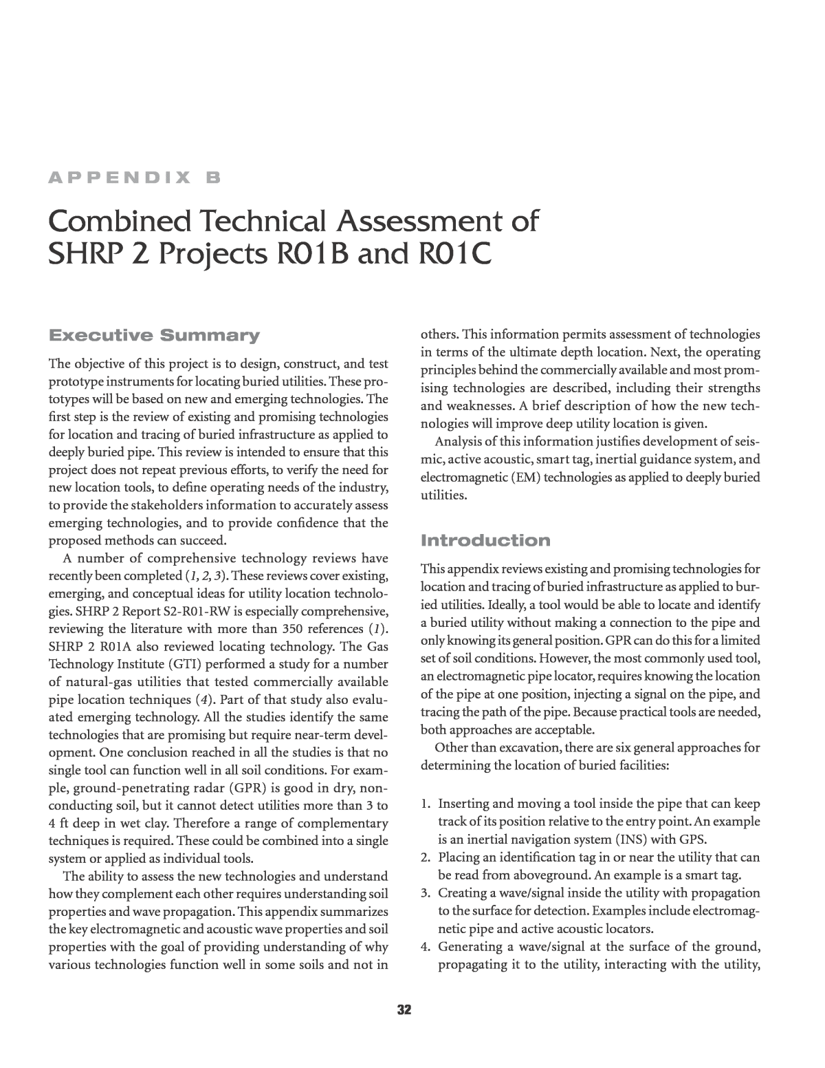
42 depth of penetration. The depth of the object is calculated by multiplying the travel time by the wave velocity. Thus, errors in the velocity affect the accuracy of depth determination. However, the lateral location of the pipe is not affected. The depth of detection depends on the soil conductivity, the power of the transmitter, and the sensitivity of the detector. As illustrated by Equation B.5, soil effects are exponential with round-trip travel distance. Because much infrastructure is buried in highly attenuating soil, additional locating tech- nologies are needed to complement GPR. GPR works best in sand and has the most difficulty in highly conductive soils, such as wet clay. Electromagnetic Pipe Locators An electromagnetic pipe locator works by detecting the mag- netic field generated by current flowing through a metal util- ity or a tracer wire. This current can be injected via direct connection or by induction into the pipe. An operator walks along the suspected path of the pipe carrying an instrument that can detect magnetic fields. Alternatively, the magnetic fields can be created in a sonde that is pushed through the utility. Sondes are used in nonmetallic conduits. The lateral range of the sonde is limited, so the operator must keep close to it as he follows its path. It is also possible to use a passive technique without coupling a tracer signal into the pipe. The passive technique relies on ambient electromagnetic signals created by radio and electric power lines and by other ground currents that follow the pipeline. However, if the ambient sig- nal is not present, the pipe cannot be found. In the active EM technique, it is necessary to create an electric current in the pipe. Thus, only metal pipes or cop- per wires placed near the pipe can be detected. The resulting alternating current creates a detectable electromagnetic field along the pipe. Ideally, the magnetic field is cylindrical, with the pipe at its center. However, the field is not always cylindrical, especially at pipe bends. Most EM pipe locators are two-piece systems: one to induce the field, and the other to detect it. The induction unit is placed at a known pipe location. The detector is moved over the suspected location of the pipe. In theory, direct currents could be used. In prac- tice, they are not used because alternating currents are eas- ier to detect. The magnetic field oscillates at the same frequency as the current. The frequencies used range from 50 Hz to 480,000 Hz. The amount of current on the pipe, not the voltage, deter- mines the magnitude of the magnetic field. In order to con- duct current, there must be a complete loop or path. The metal pipe or tracer wire provides one path. The soil provides the return path. Both the dielectric constant of the soil and its conductivity affect the return path. The soil surrounding the pipe behaves as if there were a series of small capacitors attached to the pipe. The larger these “capacitors” are, the easier it is to couple current into the pipe. Capacitance increases with the surface area of the pipe. Thus, the pipe diameter affects the distance a signal will carry. A higher soil dielectric constant will also increase the capacitance. Higher soil conductivity improves the functioning of the soil as a return path. Although higher dielectric constant and conduc- tivity increase the amount of current coupled into the pipe, they also make it easier for the current to drain away as the current flows along the pipe. The same signal strength will leak away over a much shorter distance from a large pipe than from a small one. For the same signal strength, a higher-frequency signal will decay away faster than a lower frequency. If the pipe is bare or has holidays in the coating, higher-conductivity soil will also drain away the current creating the signal. Many locators provide a choice of frequencies so that the operator can optimize the instrument for the conditions. The locating instrument uses a coil of wire for each sen- sor. The magnetic fields generate a voltage in each coil. Two coil orientations can be used to detect either a peak in the signal or a null over the pipe. A peak is measured over the pipe when the axis of the coil is oriented parallel to the ground and perpendicular to the pipe. In ideal conditions, the magnetic field surrounding the pipe is cylindrical, with the strongest signal directly over the pipe, as illustrated on the left side of Figure B.5. For deeply buried pipe, the variation in signal strength as a function of distance from the pipe on the surface of the ground is small, and precise pipe location is difficult. In such cases, the null method, with the axis of coil oriented perpen- dicular to the ground, can be used. In the null method, the signal drops to zero at three locations—far from the pipe on each side and directly over the pipe. The relationship of the measured null to the actual location of the pipe in the null Peak method Null method Figure B.5. Comparison of peak and null pipe location signals.

43 method can be skewed when interfering signals from adja- cent pipe are present. In such cases, the peak and null signals do not occur in the same place. The best locating results are obtained when the current lead is connected directly to the pipe. For cases where this is not possible, electromagnetic induction is used to couple cur- rent into the pipe. The higher the induction frequency, the more signal is coupled into the pipe. Another advantage of higher frequencies is that it is easier for them to jump across insulating joints. Higher frequencies have the disadvantages of jumping from the pipe being located to adjacent piping and attenuating faster. As discussed above, many factors enter into the ability to locate pipe. Because of those factors, the depth to which EM locators work is a difficult question to answer. As part of a confidential survey of natural-gas utilities on issues related to EM location, GTI asked at what depth they begin experienc- ing problems with accuracy in locating facilities. The answers ranged from 6 to 14 ft, depending on the installation, type of pipe, and the soil conditions. Magnetic Pipe Locators Magnetic pipe locators detect the static magnetic field sur- rounding a ferromagnetic object. When these types of utili- ties are in the presence of the earth’s magnetic field, a disturbance in the field is generated that can be detected by magnetometers. Such a field has north and south poles. The field is created by residual magnetism on the object, or it is induced by the earth’s magnetic field. Magnetometers are passive devices that respond to ferrous materials only. How- ever, magnetic detection of buried power cables is also pos- sible because those cables emit magnetic fields. In practice, the magnetic field generated by buried power cables is often distorted to some degree because of the presence of magnetic minerals in the soil, surrounding metallic pipes, and other power cables in the vicinity, resulting in several superimposed fields. Several types of magnetometers are available for use. Rela- tive to other metal detection technology, magnetometers typically perform better for large, deep ferrous utilities. One type of magnetic locator has one sensor, and the operator must detect changes in the absolute magnetic field. Another version of the instrument has two sensors, called gradiome- ters, which are separated by a fixed distance. A signal is identi- fied when the magnetic field strength at the two sensors is different. This configuration allows the gradiometer to per- form with greater tolerance to cultural interference and improves the ability to detect smaller ferrous utilities. The range of detection for magnetometers is strongly dependent on the strength of the field. Electromagnetic Induction Metal Detectors Electromagnetic induction (EMI) metal detectors work either by rapidly turning the current on and off or by using a sinusoidally varying current within a coil on the instru- ment. This varying current generates a changing primary magnetic field into the ground and induces electrical eddy currents in any nearby metallic objects. This secondary magnetic field is then measured and used for the detection of buried metallic utilities. EMI metal detectors differ from magnetometers in that they are not limited to the detection of only ferrous metals but rather may detect any conductive metal. In addition, EMI detectors are usually less affected by ambient conditions than are magnetome- ters. The two main types of EMI metal detectors are time- domain electromagnetic induction (TDEMI) detectors and frequency-domain electromagnetic induction (FDEMI) detectors. Time-Domain Electromagnetic Induction TDEMI uses a coil of wire parallel to the surface of the ground to create an electromagnetic pulse. This pulse temporarily induces eddy currents in conductive objects. After the pulse is turned off, the electromagnetic fields created by the decay- ing eddy currents are detected. The magnitude and rate of decay of the fields depend on the electrical properties and geometry of the medium and any subsurface objects. The time of arrival may give information on the depth of sub- surface metallic bodies. The currents in the earth decay or dissipate first, followed by the induced currents in metallic objects (see Figure B.6). In Figure B.6, the top series shows square-wave pulses of the transmit signal, which decay at a rapid pace when no conductive object is present. The bottom trace shows the extended decay observed from a conductive object. Arrows indicate a single time-gate measurement. Multiple time- gate measurements may be made throughout the decay period. Figure B.6. Operation of a TDEMI.

44 One version of this technology is being developed by Underground Imaging Technologies (UIT) as part of their digital multisensor system. This system incorporates both TDEMI and GPR methodologies. EMI is complementary to GPR because it is more useful in soils with high clay/ moisture content. The TDEMI component of the system consists of several transmit (Tx) and receive (Rx) coil pairs. It has fully programmable Tx and Rx parameters. As usu- ally configured for characterizing buried objects, it mea- sures the EMI decay from 0.04 ms to 25 ms. In detecting subsurface utilities, different-size pipes display different response characteristics. The wide range of response behav- iors depends on the Tx/Rx configuration, which reflects the effects of different combinations of transverse and axial response components. The basic mono-static EMI response for a metal pipe or conduit occurs in two stages. As the primary field shuts off, eddy currents are excited at the surface of the object and then decay rapidly as they diffuse into the object. During this phase the EMI response decays algebraically. As the eddy cur- rents spread throughout the object, the response shifts over to an exponential decay whose rate is determined by the physi- cal properties of the object (diameter, wall thickness, mag- netic permeability, and electrical conductivity). Different pipes or conduits have different combinations of algebraic and exponential decay parameters, and these parameters vary depending on how the line is being excited. The complete set of the sensor array data can be processed using EMI inversion algorithms to determine the basic set of parameters that fully characterize a utility line’s EMI response. The complete set of response parameters forms a unique feature vector that may be used for reliable identification and classification of under- ground utility lines. Frequency-Domain Electromagnetic Induction The basic operating principle of the FDEMI method involves a transmitter coil radiating an electromagnetic field at one or more selected frequencies to induce an electrical current (sec- ondary EM field) in the earth and subsurface objects. Depend- ing on the size of the instrument and the frequencies generated, the system can detect metallic objects at varying depths and sizes. Because the signals from the subsurface metallic objects are recorded during a time when the primary signal is still on, these instruments measure the induced currents of the conduc- tive materials differently than the time-domain instruments. FDEMI instruments measure differences in the phase and amplitude between the received signal and the transmitted sig- nal. The presence of subsurface metallic items results in changes in the measured parameters. Acoustic Locators Acoustic locators use sound waves to detect the location of the pipe. Several approaches are in various stages of development. Active Acoustic Detection In the active acoustic technique, a known signal is injected into the medium being carried by the pipe. The signal can be generated by several methods, including an acoustic driver connected to the service of a natural-gas line, a water ham- mer generated at a hydrant, or an acoustic driver hanging in a sewer manhole. The acoustic wave propagates through the medium in the pipe, not along the pipe wall. However, as the signal travels in the fluid, a portion of the signal couples into the pipe wall, causing it to vibrate. These vibrations propa- gate to the surface of the ground, where they are detected. Figure B.7 is a schematic of a two-sensor version of the active acoustic technique. A similar approach performs passive detection of the acous- tic signatures of various utilities. However, instead of injecting a signal into the medium inside the pipe, the passive tech- nique uses preexisting sounds. Passive noises include flow noise generated by natural gas or water flowing through the pipe. Because the frequency ranges are similar, the passive and Small vibrations from the pipe Two sensors on an a frame detect the vibrations Acoustic signal injected into the pipe As it travels in the gas, the acoustic signal vibrates the pipe walls Figure B.7. Sound injected into the gas in the pipe causes the pipe to vibrate. The resulting waves radiate to the surface, where they are detected.

45 active techniques can be implemented with the same sensors, signal-processing hardware, and readout display. The difference is that the active technique requires injection of a signal. The passive approach has the advantage of not needing access to the inside of the pipe. The disadvantage is that there is no guar- antee a useful signal is present. The commercial application of the active acoustic technique has been directed at locating plastic natural-gas mains. Radiodetection and Metrotech previously marketed acous- tic pipe locators that were able to locate plastic pipe buried a few feet deep. A French company, MADE, is currently marketing a similar acoustic locator called the Gas Tracker. The Radiodetection unit used frequencies of 250 and 500 Hz. As the discussion on acoustic attenuation in soil illustrated, such frequencies limit the depth of penetration. The use of much lower frequencies should extend the depth of detection. An approach in the development stage uses moling equip- ment to generate the acoustic signal. Figure B.8 is a schematic of this approach. An array of sensors is placed near the sus- pected location of the pipe. Impact vibrations from the mole are used as the signal source. Some of these vibrations propa- gate directly to the sensors. If a pipe is present, some of the vibrations also reflect from the pipe to the sensors. Cross- correlation is used to determine the presence and location of the pipe. This technique uses frequencies near 1,000 Hz with application to pipe a few feet deep. Seismic Detection Seismic detection of buried structures is a well-developed technique used to survey for water table, bedrock, oil-bearing structures, and geologic layers of interest. Seismic waves are generated at the surface of the ground. As illustrated in Fig- ure B.9, these waves propagate to the geologic structure, where a portion of the waves reflects back to the surface of the ground. This approach operates in the far field, which means the distance to the structure is large compared to the wavelength. The equipment is expensive. The analysis tech- niques are not directly applicable to detection of “near- surface” structures—structures within tens of feet of the surface—for two reasons. First, the surface soil properties are different than deeper rock. Second, buried utility structures are in the “near field” where the wavelengths are similar to the distance to the objects. This complicates the signal analysis. Sonar-type approaches for locating small-diameter pipe 3 or 4 ft deep have also been tried. An acoustic wave is gener- ated directly over the pipe. It travels to the pipe, where some of the sound is reflected back to the surface. These approaches have been only partially successful because the 1,000-Hz fre- quencies needed to see the pipe are strongly attenuated and because the soil has not stopped vibrating from the initial generation of the sound wave before the highly attenuated wave returns. Another approach is under development to detect and locate sewers and is part of the proposed development work of this project. Figure B.10 is an illustration of this approach. Two sound generators are used. One large-amplitude source creates horizontal shear waves. The second creates both horizontal and vertical shear waves. The combination obtains information on the velocities of sound at different depths in the soil, which in turn is used to determine the loca- tion and depth of the pipe. Mole Sensors Figure B.8. The moling equipment creates acoustic waves that reflect from the pipe and also travel directly to the sensors. Acoustic generator Sensors Sound waves Buried structure Figure B.9. Seismic waves can reflect from buried structures and be detected at the ground surface.

46 Inertial Navigation Internal mapping starts at a known location of the buried util- ity, inserts an instrument into the pipe, and moves the instru- ment through the pipe. New and emerging inertial navigation system (INS) instruments use a combination of accelerome- ters, gyroscopes, and odometers to measure the distance the tool has moved and the changes in orientation of the tool. Accurate measurements of angles and distances are used to calculate the relative position of the tool to the entry point. These values are stored and downloaded to a laptop computer. A 3-D map of the pipe position is obtained. In principle, INS can be used from one entry point and travel for long distances through the pipe. However, the range of an inertial mapping tool is limited by cumulative error; the accuracy slowly degrades with distance from the insertion point. One of the more accurate INS tools quotes tolerances of +0.25% in the x and y (lateral position) and +0.1% in the z (depth). This results in a possible position offset of 12 in. in 400 ft, and 5 ft after a distance of 2,000 ft. The accuracy of INS location will improve as angle-measuring sensor technology becomes more accu- rate. Accuracy can also be improved if the locations of the pipe are known at one or more discrete positions. Smart Tagging Another approach to buried utility location is to bury indica- tors, or smart tags, that can be interrogated from the surface of the ground. Tags could be installed inside the pipe with robotics or attached to pipes before being directionally drilled into the ground. A reader would be used to determine the facility location. Systematically adding tags during other operations would make facility location easier in the future. Smart tags contain information that can be interrogated from aboveground. One version of these, RuBee-enabled under- ground wireless pipe location and relocation systems (RuBee tags), is being developed and commercialized by Visible Assets, Inc. (VAI) for a broad range of applications. RuBee tags are based on the open IEEE 1902.1 standard. IEEE 1902.1 is a wireless, two-way, peer-to-peer transceiver protocol. They may be simple identity tags with only an IP address, or they can have a four-bit processor with 500 to 5,000 bytes of static memory, optional sen- sors, and signal-processing firmware. Previous attempts to use buried radio frequency identification (RFID) detection have not been successful, in part because the high frequencies used cannot penetrate deeply into the soil. RuBee is not like RFID, because it is a packet-based protocol and operates at a frequency (131 KHz) that can be detected even when deeply buried. The low opera- tional frequency permits long battery life—up to 20 years on a coin-size CR2525 lithium battery. The range can be a few feet to more than 70 ft, depending on tag and antenna design. Read/ write ranges can be 40 ft underground. With extra antennas, RuBee can provide 3-D localization. The tags are low-cost and can operate in harsh, underwater environments. The project proposes to create two prototype tag products focused on location of deeply buried facilities. These tags will be waterproof, explosion proof, and designed for an average underground life of 15 years, with a range of 35 ft. Tags will be programmed with three-axis location data and, optionally, other relevant information about the buried assets, and will have 500 bytes of onboard read/write storage. One prototype version is aimed at new construction and retrofit burial. The second version of these tags would be attached directly onto a pipe, either inside or outside. The form factor will be con- formal to the shape of the pipe itself, with the long-term goal of manufacturing the tags as part of the pipe. The project also proposes to create two handheld reader/ locators. One RuBee reader and writer will be able to read data from the tag and also add useful information to the tag, such as GPS coordinates, pipe depth, date and time of instal- lation, pipe type, size, content, and other field-critical data. The second reader/locator would have a longer range and only read data from the smart tag. Infrared Thermography Infrared thermography is a technique that detects tempera- ture differences on surfaces. In concept, leaks and product Figure B.10. Acoustic S-waves offer promise for locating deep utilities.

47 flowing in the pipe create temperature differences between the pipe and ground. These in turn create a temperature field at the surface of the ground, with the highest or lowest tem- perature above the pipe. The technique has had limited suc- cess in locating water leaks, voids, and other similar anomalies. However, the temperature gradients at the ground surface are small for shallowly buried pipe. They became even smaller as the pipe depth increases. The technique has little potential for detecting deeply buried facilities. Capacitive Tomography Imaging Capacitive tomography is a technology in the early stages of development with potential for detecting buried facilities. One usually thinks of a capacitor as composed of two parallel, charged conducting plates separated by a small distance (see the top portion of Figure B.11). The space between the plates may be filled with a dielectric to increase the capacitance. Normally, the dielectric material is uniform. Any variations within the dielectric cause variations in the local electric field. The capacitive tomography sensor is composed of many plates, all in the same plane (see the bottom portion of Fig- ure B.11). The technique applies an alternating current between each set of plates and measures the resulting steady- state electrical impedance under each plate. Variations among the impedances indicate the location of buried pipe. Capacitive tomography depends on differences between the relative dielec- tric constant and the electrical conductivity of the soil. Fre- quency range is much lower than GPR (100 kHz to 400 kHz); therefore, penetration depth is better. The image resolution is set by plate size and spacing, not frequency. Time of flight is not measured, so no high-speed signal processing is required. Experiments indicate that the capacitive tomogra- phy technique functions best in wet soil and has difficulty in dry soils—the opposite of GPR. The sensor sees deeper by decreasing the frequency. However, the lower frequencies also detect all the material between the surface down to the maxi- mum depth. A method is needed to separate the near-surface features from the deeper features. Development issues include trade-offs between the size of each plate and the ability to detect changes in dielectric properties. The smaller plates required for higher resolution have very small capacitances, creating measurement problems. discussion of Advantages of proposed Technologies The wide range of pipe materials, diameters, and burial depths combined with the wide range of soil properties and their effects on pipe location technologies means that no single technique will work in all soil types. This is especially true for deeply buried facilities. A complementary set of tools is required. The goal of this project is to develop several proto- type tools that can be used in proof-of-concept tests. This section summarizes how each proposed technology improves on the existing art. Smart Tags One approach to buried utility location is to bury indicators, or smart tags, that can be interrogated from the surface of the ground. Marker ball tags composed of a resonant coil/capacitor circuit have been used for shallow depths for many years. Previous attempts to use buried RFID detection with more information at deeper depths have not been successful, in part because the high frequencies used cannot penetrate deeply into the soil. VAI proposes to create two prototype tag products that can be used at depths of 35 ft. These tags will be based on the open IEEE 1902.1 standard, referred to as RuBee tags. RuBee is not like RFID, because it is a packet-based protocol and operates at a frequency (131 KHz) that can be detected even when deeply buried. The tags for this project will contain 500 bytes of onboard read/write storage. The project also proposes to create two handheld reader/locators. One RuBee reader and writer would be able to read data from the tag and also add useful information to the tag, such as GPS coordinates, pipe depth, date and time of installation, pipe type, size, content, and other field-critical data. The other will work at greater depths but will only read data. Inertial Navigation Systems An inertial navigation system (INS) inserts a tool into the subject pipe. Sensors detect the orientation of the tool as a function of distance as it moves through the pipe. These data are used to calculate the position of the tool with respect to No dielectric Nonuniform dielectric In capacitive tomography, the plates are in the same plane. + + + + + + + + + + + - - - - - - - - - - - - - - - - - - - - - - + + + + + + + + + + + + + + + + + + + + + +- - - - - - - - - - - Figure B.11. In a typical capacitor, the electric field between two parallel plates is perpendicular to the plates. In capacitive tomography, the plates are in the same plane.

48 the entry point. For this tool, GTI will work with Geospatial and their commercially available Smart Probe to make opera- tional improvements in three areas. “Live” Insertions Requiring the utility to be shut down and taken out of service before running inertial mapping tools is a significant limita- tion. Many pressurized lines cannot be shut down because of the critical nature of their services. Inserting the INS tool through a small hole in the pipe at operating pressure (called “hot tapping”) will increase the practicality for locating deeply buried utility lines. GTI has developed hot-tap tech- nologies for other applications. This experience will be lever- aged to develop prototype fittings and techniques for live inertial mapping tool insertion. Smart Tag Internal Benchmarking The range of inertial mapping tools is limited by cumulative error. Because the angular measurements have error, the accuracy of the calculated position slowly degrades with dis- tance from the insertion point. Corrections can be made if the true location of the pipe is known at discrete positions along the pipe. Smart tags can be installed at selected loca- tions and used as a benchmark to enhance the accuracy of inertial mapping. There is another potential synergy between inertial mapping tools and smart tags. If the inertial mapping tools could also be used to install smart tags on the interior of a pipe wall, relocating these facilities in the future would be greatly simplified. One part of the smart tag project is the development of tags for deep-pipe applications. Another part is development of prototype tags that can be installed on the interior surface of the pipe during mapping. Small-Hole Insertion Excavation and restoration costs are a significant factor in determining the practicality of using inertial mapping tools. Developing installation techniques that reduce the size of the excavation, and therefore reduce the total cost of use, would also increase the feasibility of this technology. Keyhole technol- ogy is one of the largest research and development programs at GTI. It includes pavement cutting, vacuum excavation, and long-armed tool development, as well as protocol and stan- dards development. The project team will create prototype long-armed tools and attachments to allow the inertial map- ping tools to be installed in a keyhole. Electromagnetic Noncontact Technology EM pipe location using a sinusoidally time-varying current is the most widely used technique for locating buried metal pipe. A current is injected into the pipe, and an operator walks over the pipe carrying a detector. The depth of applica- tion is typically 10 ft or less. At some sites, metallic and non- metallic facilities are buried too deeply for conventional EM pipe locators. However, where manholes provide access to nonmetallic facilities, INS can be used to map them. How- ever, this will not detect adjacent metal pipe. GTI proposes to develop a prototype tool that can be passed through a nonmetallic pipe and scan the surrounding soil vol- ume for metal pipes. In this EM technique, a rotating EM field is projected into the soil. The projected field induces eddy cur- rents in metallic objects, which in turn produce a detectable field. The rotating field is generated by a set of driven coils, so phased as to gradually rotate the driven field through 360° about a central axis. The primary frequency of the EM signal and the rate of the field rotation are independently adjustable. One or more sensing coils monitor the EM field as it rotates. Metallic materials within the range of the instrument disturb the EM field and are detected by the sensing coils. This will provide knowledge on piping within approximately a 10-ft radius of the sewer. Because the field is rotating, the tool will give the direction to the adjacent pipe, and more than one pipe can be detected. The prototype could also be lowered into a vertical borehole and used to scan the surrounding volume. The GTI EM innovation prototype will be designed to be synergistic with technologies provided by other research partners, specifically smart tags and INSs. In addition to the EM frequencies required to locate buried metallic facilities, the prototype will scan frequencies used for several types of buried radio frequency (RF) location tags. The EM innova- tion prototype will be able to detect the presence of passive RF tags that have been used by utilities for several decades. Additionally, the prototype will be able to both detect and interact with the RuBee (IEEE 1902.1) smart tags being pro- duced by VAI for this project. The EM innovation prototype will also be able to be used in conjunction with the INS and GPS technologies provided by Geospatial. The use of INS technology will greatly simplify the odometry portion of the work aboveground and when used in buried ducts. Unlike traditional EM locators, the EM innovation proto- type will detect metal piping without injecting a current into the pipe. The direction to the pipe is part of the information generated. Thus, the new tool will also be able to be used at the surface of the ground to detect piping. There would be advantages where parallel pipes exist. Conventional EM loca- tors typically predict the existence of one pipe. With the new tool, signal returns from more than one direction will indi- cate the presence and location of two or more pipes. Seismic Reflection Technology The seismic reflection approach will be developed by UIT. The approach is to launch acoustic waves at the surface of the

49 ground. These waves will propagate to the pipe and reflect to sensors on the surface of the ground. This development will be performed in collaboration with similar work proposed for the R01B project in which initial measurements of seismic properties of soils will be made to optimize receiver specifica- tions. The R01B project is developing an S-wave seismic sys- tem for mapping dense, shallow networks of utilities. The R01C project will use similar techniques and will develop instrumentation and analysis techniques that could be com- plementary to detect and image deeper pipe. The proposed technique improves on previous technology by using horizontal shear (SH) and vertical shear (SV) waves to detect the pipe. When compared with longitudinal acoustic waves of the same frequency, S-waves have a shorter wavelength. The shorter S-waves will yield improved pipe imaging. With respect to the detection of small objects and utility targets, S-waves offer several distinct advantages over com- pressional waves: • Propagation velocity. S-waves travel considerably slower than P-waves in unconsolidated soils. In many cases, the S-wave velocity is only about one-quarter that of the P-wave velocity. Given that the relationship between fre- quency, velocity, and wavelength is linear, the end result is that S-waves have much shorter wavelengths than P-waves in the same soil medium. This difference can yield up to 4 to 8 times better resolving power for S-wave detection of small targets, depending on soil properties, in comparison with P-waves when operating in the same frequency range. • Voids. S-waves cannot propagate through fluids. A much higher percentage of energy is reflected from a void space for S-waves than for P-waves. Because very nearly all utili- ties are rigid pipes with an internal void space containing gas or liquid, S-waves are much more effective in detecting these types of objects. • Particle motion polarization. Horizontally polarized SH- waves in particular exhibit higher reflections from elon- gated objects, such as pipes, when the polarization is parallel to the pipe-axis alignment than when transverse to the alignment. Therefore, SH-waves can provide more sen- sitive detection of small-diameter pipes when the general pipe alignment direction is known and used in the scan- ning process. • Wave-type conversion. SH-waves do not undergo wave- type conversion and attendant energy partitioning between shear and compressional waves when transmitted through or reflected from horizontal contrasting interfaces. There- fore, with the polarization parallel to any intervening soil- layer interfaces, all the transmitted SH-wave energy remains available for detecting deeper objects. • Surface waves. “Pure” SH-waves, not combined with con- taminating P-waves or vertically polarized SV-waves gen- erated at the surface, do not excite surface (Rayleigh) waves that can interfere with detecting and recognizing shallow SH-wave reflections. • Ambient noise. Very nearly all the ambient noise generated by vehicular traffic and walking personnel, construction activities, and other sources of vibration is either P-wave or surface wave in nature. Therefore, SH-wave sensors have a much better ability to discriminate against most types of ambient noise than do their P-wave counterparts. Changing from geophones to accelerometers will increase the frequency range available, which will help in the imaging. The increased frequency range combined with improvements in measurement system hardware and data processing meth- odologies should produce a system that is more field efficient for this project’s purpose, less time consuming, less costly, and, most important, more effective at finding the deep tar- gets. Electronically driven impact sources of two different sizes will be used for the signal source. The larger source will be used to collect lower-frequency data for large-scale veloc- ity analysis, and the smaller source will be used to collect shal- low velocity data, as well as reflection data, for imaging the target. Having a more complete knowledge of velocity over the depth range of interest allows accurate calculation of tar- get location and depth. Active Injection Acoustic Technology GTI will develop a complementary acoustic technique for locating deeply buried pipe. A pulsed acoustic signal of known shape is generated in the interior of the subject pipe. This acoustic wave propagates through the medium in the pipe, not in the pipe wall. However, as the signal travels in the fluid, a portion of the signal couples into the pipe wall. Vibrations from the pipe wall propagate to the surface of the ground, where they are detected. This approach has two advantages. First, the sound waves travel only one way (from the pipe to the surface rather than from the surface to the pipe and back). Because attenuation is exponential with distance traveled, one-way propagation yields lower signal attenuation. Second, the sound waves are not imaging the pipe; therefore, lower frequencies can be used, again reducing attenuation and increasing the ability to detect pipe. The prototype will measure the arrival times of the signals (time of flight). Because the signal is known, powerful signal- processing techniques can be used to discriminate the pipe location signal from background noise. The time-of-flight technique is relatively insensitive to variations in coupling between the sensor and ground. In addition, GTI will use the same prototype tool to per- form passive detection of the acoustic signatures of various utilities. Passive noises include flow noise generated by natu- ral gas or water flowing through the pipe or acoustic hum generated in electrical cables.

50 Seismic and Acoustic Compared One of the overall goals of the project is to develop a suite of complementary technologies. The seismic reflection method has the advantage at locations where the buried facility is inaccessible. The active method has some advantages over the seismic reflection method in those instances where there is access. Because the acoustic signal only travels from the pip- ing to the ground surface, it suffers less attenuation. The active signal is injected into a particular pipe; therefore, the pipe is positively identified. The signal originates in the pipe instead of reflecting from its surface, relaxing the require- ment that the wavelength must be scaled to the pipe diameter. The active method could use lower frequencies, which suffer less attenuation to achieve extra depth. The passive acoustic technique is expected to be effective on live electrical cables. GPR and Seismic Compared GPR has been the dominant utility location method used to date. It has quite effective resolution, it is fast to deploy, its raw data displays are reasonably straightforward to interpret, and it is reliable when ground penetration to the desired depths is practical. The problem is that GPR impulses, typi- cally in the 80- to 500-MHz spectral range, do not penetrate to useful depths in a variety of soils common to utility burial environments: • Clay; • Caliche; or • Wet or saline soils. In short, the method does not work well when the soil is electrically conductive. Seismic methods have been successfully used in the past to locate large utilities. In particular, those methods that used SH-waves have enjoyed the most success. The principal sub- surface applications using SH-waves have employed the seismic reflection technique in locating caves, sinkhole voids, tunnels, and large underground sewer pipes. This is directly relevant to the detection of other types of utilities because most utility lines are in fact long, cylindrical targets containing either wires or fluids. In particular, the following results have been achieved using SH-wave seismic reflection methods: • Location of a 2-ft-diameter tubular cavity in limestone at a depth of 70 ft. • Location of underground coal and iron mines in New Mexico, Minnesota, Ohio, Indiana, Illinois, Iowa, Michigan, and New York at depths ranging from 100 ft to 1,000 ft. • Location of voids along the top of jointed concrete storm sewers in Texas, New Jersey, and Louisiana. • Location of large concrete pipes (>1-ft diameter) in Cali- fornia, Texas, and Louisiana at depths ranging from 10 to 50 ft. Horizontally polarized shear waves generated by a vibrator source excited by a long–time-duration, linear-sine-wave sweep signal, and later processed by correlation analysis to produce reflection pulse wavelets, have been demonstrated to be effective in extremely noisy environments, including the following: • SFO Airport, San Francisco; • Downtown cities of Los Angeles, Minneapolis, and Des Moines; • Operating oil refineries in Texas, Louisiana, and Minne- sota; and • Along the paved shoulders of interstate highways in Cali- fornia and Ohio. Figure B.12 shows a chart of estimated quarter wavelengths for GPR signals at various MHz frequencies and seismic sig- nals for various frequencies in the Hz to KHz range. Since target detection is a function of wavelength, and since the detection capability in good soils of GPR, at say 400 MHz, is quite adequate, it seems appropriate to attempt to attain the same wavelengths for seismic impulses as are produced by GPR systems. Figure B.12 uses an average value of dielectric permittivity for GPR in favorable soil and reasonable values for P-wave and S-wave velocities in near-surface soils. It is clear that if gener- ating and propagating seismic waves of sufficiently high fre- quency is the problem, then using S-waves may provide an advantage. A quarter wavelength similar to that of a 400-MHz GPR signal in average soils for GPR can be produced with S-waves in the range of 700 to 1,000 Hz in soils good for seis- mic. However, it would be necessary to use P-waves of about 3,000 Hz to produce the same quarter wavelength in those same soils. UIT, Owen, and Psi-G have experience that sug- gests generating and propagating 3,000 Hz seismic waves is very difficult. Work has been done with S-waves in depth ranges only a little deeper than is sought for normal utility mapping. Fig- ure B.13 is an S-wave reflection cross section that shows a hyperbolic signature at the location of a sewer pipe at a depth of 11.6 m (38 ft). The maximum frequency detectable for this survey was about 700 Hz using an S-wave vibrator and a geo- phone streamer. This work is at least partial proof of the con- cept of using S-waves for detection of utilities. However, the survey in the example was expensive and difficult to process and would not be acceptable for use in normal utility map- ping work as a result. On the basis of ideas under consider- ation for this project, which include appropriate modifications

51 to field methodology and data processing, it may be possible to improve the time efficiency and cost of S-wave seismic sur- veys to make them both functionally and economically useful for utility mapping. The use of multiple sensor, multiple antenna/transducer geophysical systems for improved mapping of buried utilities has been demonstrated and is used in the commercial market today. The integration of GPR, EMI, good positioning, and a 3-D workspace for first-order data fusion provide a big step forward in geophysical capabilities for mapping shallow utili- ties. Initial ideas and testing on the addition of a seismic com- ponent to the sensor package have validated the potential use of S-waves for mapping the types of targets sought for nor- mal utility mapping in soils not compatible with GPR. Quarter Wavelengths 0 1 10 100 1000 0 500 1000 1500 2000 2500 3000 3500 4000 4500 5000 5500 6000 Frequency (Seismic-Hz / GPR-MHz) Qu ar te r W av el en gt h (cm ) GPR ε =12 S-Wave Seismic V = 122 m/s P-Wave Seismic V = 608 m/s Figure B.12. Quarter wavelengths for GPR and seismic. Figure B.13. S-wave reflection cross section with highlighted location of sewer pipe at 11.6 m (38 ft).

52 Table B.4. Locating Technologies Matrix Technology Horizontal Accuracy Vertical Accuracy Factors Effecting Accuracy Ease of Use Features Examples Comments Electro- magnetic pipe and cable locators 2–12 in. 5–20% of depth Soil conditions, utility material and size, proximity of metallic struc- tures, ability to directly connect to the utility Moderate— audio and visual indica- tors require interpretation GPS integration, 2-D signals, signal quality indicators, limited data output options Metrotech, 3M Dynatel, and Heath Surelock EM locators are the industry standard for routine utility locate and mark-out opera- tions. While the devices are relatively sim- ple to use, a fair amount of interpretation is required to pinpoint the location of the underground facility. EM locators cannot locate nonmetallic utilities and are depen- dent on the presence and condition of tracing wires. Sondes 2–12 in. 5–20% of depth Soil conditions, utility material and size, proximity of metallic struc- tures, ability to directly connect to the utility Moderate— audio and visual indica- tors require interpretation GPS integration, 2-D signals, signal quality indicators, limited data output options RD, Rycom, Ridgid Sondes are an effective tool for locating plastic utility lines but require access to the internal pipe and are limited in the dis- tances that can be located. Ground- penetrating radar 2–24 in. The vertical accuracy of GPR is high if the utility can be detected. Signal attenuation can result in depth penetrations ranging from 12 in. to 10 ft. Soil moisture and conductivity, utility material and size, user experience and interpretation Low—significant training and signal inter- pretation required GPS integration, 3-D mapping output Noggin Smart- Cart, Pipe- hawk, and US Radar GPR used primarily by specialized service providers and SUE firms. Direct use by utility companies has been limited because of the high cost, training require- ments, and variable performance in differ- ent soil conditions. Acoustic and seismic locators 6–12 in. based on lim- ited testing Limited information available Soil moisture and ground cover Moderate Limited data output options MADE Gas Tracker, R01B and R01C Commercially available acoustic locators require access to either the content of the pipe (gas) or the pipe (water). The primary advantage of acoustic locators is the abil- ity to locate nonmetallic lines. GTI is developing an acoustic locator that does not require access to the pipe or the pipe contents. Magnetic locators Limited information available, but the technology is sensitive to interference. Utility size and material Moderate Limited data output options Geometrics, GEM Systems The primary application for magnetic locat- ing tools is large, deeply buried ferrous materials. Electro- magnetic induction Limited information available for utility applications. R01B Similar to magnetometers, but can locate other nonferrous materials and is less sensitive to nearby metallic structures and conductive soil conditions. Inertial navigation Very precise but drifts with increasing distances without calibration. Toler- ances are 0.25% of the distance in the horizontal direction and 0.10% in the vertical direction. Distance traveled High—minimal interpretation required Output can be formatted in CAD or GIS. Geospatial Smart Probe Inertial navigation is not technically a locat- ing device, but it can be used to map out the location of a pipe. This technology is particularly useful for deep or directionally drilled utilities. Use of the Smart Probe requires the line to be taken out of ser- vice, although developments for live applications are feasible.

53 nonplane Wave Bibliography Annan, A. P. 2005. Ground-Penetrating Radar. In Near-Surface Geophysics (D. K. Butler, ed.), Society of Exploration Geophysicists, Tulsa, Okla., pp. 357–438. Belli, K., C. Rappaport, and S. Wadia-Fascetti. 2009. Forward Time Domain Ground Penetrating Radar Modeling of Scattering from Anomalies in the Presence of Steel Rein- forcements. Research in Nondestructive Evaluation, Vol. 20, No. 4, pp. 193–214. Berkovitch, A., I. Belfer, Y. Hassin, and E. Landa. 2009. Dif- fraction Imaging by Multifocusing. Geophysics, Vol. 74, No. 6, pp. WCA75–WCA81. Elmore, W. C., and M. A. Heald. 1969. Physics of Waves. Dover Publications, New York. Fomel, S., E. Landa, and M. T. Taner. 2007. Poststack Velocity Analysis by Separation and Imaging of Seismic Diffrac- tions. Geophysics, Vol. 72, No. 6, pp. U89–U94. Foo, K. Y., P. R. Atkins, A. M. Thomas, and C. D. F. Rogers. 2010. Capacitive-Coupled Electric-Field Sensing for Urban Sub-surface Mapping: Motivations and Practical Challenges. Proc., 1st International Conference on Fron- tiers in Shallow Subsurface Technology, Delft, Netherlands, pp. 157–160. Fratta, D., A. L. Fernandez, and J. C. Santamarina. 2001. Geo- materials: Non-destructive Evaluation in Geosystems. In Review of Progress in QNDE, Vol. 20 (D. O. Thompson and D. E. Chimenti, eds.), American Institute of Physics, pp. 1048–1055. Gao, Y., M. Brennan, and P. Joseph. 2006. A Comparison of Time Delay Estimators for the Detection of Leak Noise Sig- nals in Plastic Water Distribution Pipes. Journal of Sound and Vibration, Vol. 292, pp. 552–570. Graff, K. H. 1974. Wave Motions in Elastic Solids. Dover Pub- lications, New York. Lowry, C., D. Fratta, and M. Anderson. 2009. Using Ground Penetrating Radar to Identify Processes Controlling Spring Flow in a Peat Dominated Wetland. Journal of Hydrology, Vol. 373, pp. 68–79. Mow, C. C., and Y. H. Pao. 1971. The Diffraction of Elastic Waves and Dynamic Considerations. Report prepared for USAF Project Rand. The Rand Corporation. Santamarina, J. C., K. A. Klein, and M. A. Fam. 2001. Soils and Waves. Wiley, Chichester, UK. Schroeder, C., W. Scott. 1999. Finite-Difference Time-Domain Model for Elastic Waves in the Ground. Proc., SPIE 3710, Detection and Remediation Technologies for Mines and Minelike Targets IV, 1361. Tao, L., T. Tanaka, T. Watanabe, S. Motooka, S. Murayama, and I. Yoshihisa. 1999. Ultrasonic Underground Imaging Using Amplitude Correlation Synthesizing Method. Japa- nese Journal of Applied Physics, Vol. 38, pp. 3148–3153. Yilmaz, O. 2001. Seismic Data Analysis: Processing, Inversion, and Interpretation of Seismic Data. Society of Exploration Geophysicists, Tulsa, Okla. References 1. Sterling, R. L., J. Anspach, et al. SHRP 2 Report S2-R01-RW: Encour- aging Innovation in Locating and Characterizing Underground Utili- ties. Transportation Research Board of the National Academies, Washington, D.C., 2009. 2. Common Ground Alliance. Review of NTSB Recommendation P-97-16/P-97-17, February 2003. 3. Metje, N., et al. Mapping the Underworld—State-of-the-Art Review. Tunnelling and Underground Space Technology, Vol. 22, 2007, pp. 568–586. 4. Underground Facility Pinpointing—Alternative Locating Technolo- gies Assessment. Final Operations Technology Development (OTD) Report, December 2005. 5. Durney, C. H. Introduction to Modern Electromagnetics. McGraw- Hill, New York, 1969. 6. Marion, J. B. Classical Electromagnetic Radiation, Chapter 5. Aca- demic Press, New York, 1965. 7. Miller, R. C., M. A. Attili, and P. G. Marston. Improvement in TERRASCAN Instrumentation and Techniques for Location of Buried Pipe. GRI-87/0089. March 1987, pp. 27, 79. 8. Oelze, M. L., W. D. O’Brien, Jr., and R. G. Darmody. Measurement of Attenuation and Speed of Sound in Soils. Soil Science of America Journal, Vol. 66, 2002, pp. 788–796. 9. Huebler, J. E., B. K. Campbell, and N. C. Saha. IGT Acoustic Plastic Pipe Locator. Final Report for Southern California Gas Company, April 1990.