
Inception, Development, and Noise of a Tip Vortex Cavitation
L.Briançon-Marjollet, L.Merle (Bassin d'Essais des Carènes, France)
ABSTRACT
Experiments were conducted on a large hydrofoil, of elliptical planform and NACA 0020 cross section, to test the influence of the water quality on: the cavitation map, the diameter of the cavity within the tip vortex and the noise measurements. Water is characterised in term of oxygen and freestream bubbles content. We observe strong effects of the freestream nuclei content on the cavitation map and on time variation of the vapor core diameter. All results at cavitation inception can be correlated by introducing a corrective term calculated from the measured water quality. The growth of the diameter with time, as well as the hysteresis at the desinence cavitation, can be interpreted taking into account the non condensible gas diffusion. Acoustic data are presented in term of counts of acoustic peaks, or in term of peculiar frequencies associated to the vapor tube. These results are confronted with the visual data and modes of deformation of the vapor tube are given.
NOMENCLATURE
|
a |
radius of the cavitating vortex core |
|
c |
maximum chord length |
|
Cl |
lift coefficient related to the surface of the foil |
|
Cp |
pressure coefficient at the vortex axis |
|
D |
cavitating core diameter |
|
F |
frequency |
|
f |
focal lenght |
|
H |
hysteresis |
|
i |
angle of attack of the foil |
|
K(x) |
experimental coefficient |
|
N |
aperture |
|
P |
pressure of the inlet flow at the middle of the test section |
|
Pc |
critical pressure of nuclei |
|
Ps |
susceptibility pressure of the fluid |
|
Pv |
vapour pressure of water |
|
r |
radius |
|
Re |
Reynolds number based on the maximum chord length |
|
t |
time |
|
T |
surface tension |
|
V |
free stream velocity |
|
Vt |
tangential velocity |
|
x |
abscissa |
|
γ |
Euler constant |
|
Γ |
circulation |
|
ρ |
volumic mass of liquid |
|
σ |
cavitation number |
|
σ0 |
cavitation number at the beginning of the developed cavity |
|
∞ |
far from the vortex axis, in the perpendicular plan of the centerline vortex |
|
PSD |
Power Spectral Density |
|
G.T.H. |
Grand Tunnel Hydrodynamique |
|
CSM |
Cavitation Susceptibility Meter |
1.
INTRODUCTION
Even if the cavitation of tip vortex was studied for a long time by many authors, some aspects had to be clarified. The fact that this type of cavitation is closely link to propellers conduct to have a special attention on it. It's Reynolds number dependance was studied. However, some questions remain: what is the best way to perform and interprate model tests in
order to extrapolate the results to full scale? In many papers, authors indicate that oxygen content acts on cavitation inception ([2], [3], [6], [9]) and on desinence cavitation[13]. We could ask if there is a best water quality for model tests. But the above mentionned studies do not permit to quantitatively correlate a parameter describing water quality and a cavitation number.
Many studies were conducted on different French tests facilities during the Action Concertée Cavitation. The aim was a better understanding of tip vortex roll-up and of associated cavitating phenomenon ([ 7], [8], [11]). Due to the fact that the water tunnel, the Grand Tunnel Hydrodynamique G.T.H., permits us to control the oxygen content independently from the freestream nuclei content, the Bassin d'Essais des Carènes was in charge of studing relation between oxygen content, freestream nuclei content and inception, development and desinence of cavitation [11].
The aim of this paper is first to recall the main results obtained during these tests. For the cavity within the tip vortex-roll up, a law was yet proposed as a function of the Reynolds number for a single water quality at the desinence cavitation [8]. We will see in this paper, how all the data for cavitation inception can be fitted on a single curve when taking into account freestream nuclei.
The diameter of the cavity within the vortex was also measured. This allowed to appreciate how the water quality affects the development of cavitation. Thus, the hysteresis at desinence can be explain by diffusion of non condensable gas as expected by Holl [13].
At the inception of the cavity, we observe bubbles growing in the center of the tip vortex for special water quality. These bubbles, captured by the vortex, could grow by diffusion of non condensible gas or could explose by vaporisation of liquid. We are particulary interested in the acoustic noise and, in the following, we will call cavitation inception, a phenomenon with two particularities: we can locate the tip vortex in the flow visually, and there is a raise of the acoustic noise.
For developed cavitation, specific frequencies were extracted in the spectrum signal. These frequencies are compared with the frequencies of modal deformations of the cavity.
2.
EXPERIMENTAL SETUP
2.1
Flow parameters
Experiments were conducted in the G.T.H. [5], in the square test section of 1.14 m width, 1.14 m high and of 6 m long. The studies were made with an elliptical planform hydrofoil, the maximum chord is 475 mm and the half-span equals 753 mm (the aspect ratio is 3.8), the cross-section is a NACA 0020.
The tunnel permits us to control the inlet velocity between 2 m/s up to 20 m/s with an accuracy of 0.2%. The pressure level varies between 2.104 Pa up to 4.5 105 Pa, with an accuracy of 0.5%. The cavitation number σ is defined as:
(1)
with P, the total inlet pressure in the plane of the tip of the hydrofoil, Pv, the vapor pressure of water, ρ the volumic mass of water and V the inlet flow velocity. The precision of σ is 1%.
The oxygen content is controlled between 25% up to 160% of saturation and is measured with an oxygen probe. The flow can be seeded with nuclei through injectors located upstream the tunnel nozzle. A Cavitation Susceptibility Meter based on a centerbody venturi (called VAG) measures the nuclei distribution in the fluid. Hence, the number of nuclei with a given critical pressure is known for each test configuration. Several nuclei injections patterns were tested. They are characterised by a specific susceptibility pressure, a concentration and a distribution in the test section. Hereafter, the higher Ps (lower tension) corresponds to the water with ‘big' bubbles, then we have a medium Ps for ‘small' bubbles and the water without injection have the lowest Ps (higher tension). For more details, see [3].
Cavitating data were collected with the two testing configurations of nuclei presented below.
2.2
First configuration
The hydrofoil is mounted vertically at the top of the test section (Figure 1). The angle of attack is changed
by hand with a precision of ±0.1°. Measurements of the tangential and axial velocities in the subcavitating vortex were carried out at several positions along the axial distance with a LDV system, for different velocities and angles of attack [8].
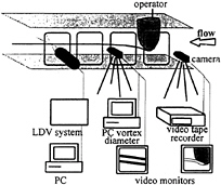
Fig. 1: experimental facility, 1st configuration. Location of apparatus is not represented.
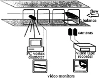
Fig. 2: experimental facility, 2nd configuration. Location of apparatus is not represented.
A map of the observed cavitation versus the angle of attack is drawn by looking at video records, for velocities between 5 m/s up to 15 m/s by step of 1 m/s. The water quality corresponds to a low oxygen content of 30%, without nuclei injection. The pressure and the flow velocity are kept constant, whereas the angle of attack is slowly increased until the inception and development of the cavity. Then, the angle of attack is decreased until desinence cavitation.
Further tests were performed at particular experimental points with different oxygen contents and nuclei injections. The diameter of the vapor tube is measured with a real time image analysis method. The sound radiated by the cavitation is analysed and recorded.
2.3
Second configuration
The hydrofoil is mounted horizontally on a side wall of the test section (Figure 2). The angle of attack is controlled by a balance with a precision of ±0.01°. The influence of the water quality is largely studied in these experiments. Flows with oxygen content of 30%, 56% and 80% are studied as well as flows with several nuclei injections with an oxygen content of 30%. Again, a map of the observed cavitation as a function of the angle of attack is drawn by visualisation of video records for 3 velocities: 6 m/s, 10 m/s and 15 m/s. A more systematic investigation of the vapor tube diameter is carried out with the same image processing method as previously. The hydrodynamic coefficients are measured with the 6 components strain gauges balance. The acoustic signal is recorded and peaks are counted at the cavitation inception.
2.4
Set up for measuring the size of cavitating vortex
A special system was built using digital images from a video camera to measure the vortex size and to analyse the changes in size as a function of time and gas content. A video camera is focussed on the vortex core. The camera output is connected to a PC that records the image and calculates the mean diameter (Figure 3).
A black and white video camera with a f=300 mm focal length lens and N=2.8l aperture produces a magnification factor of 1/0.22. The video camera has a CCD sensor of 511×768 pixels, each pixel being 11µm×11µm. The PC records a full frame of the image. The images are recorded every 30 seconds and they are analysed immediately afterwards. The grey level of the numerical image is set between 0 and 255.
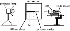
Fig. 3: image recording system.
The lighting system is an halogen projector lamp with a diffuser sheet mounted at the back of the plexiglass window of the test section. The coaxial lighting makes a shadow view of the vortex on the recorded image so that the edge of the tip vortex core is very contrasted.
The vortex core has sufficient contrast such that its contour is directly obtained by converting the greyscale image into a binary image based on a threshold range. Then the diameter and the angle of the vortex are calculated (Figure 4).
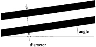
Fig. 4: binary image of the vortex core.
The selected threshold level has little effect on the calculated diameter and the maximum diameter uncertainty is 0.2mm.
2.5
Acoustic apparatus
The sound radiated at cavitation inception and for developed cavitation is analysed in two ways, one for each configuration.
The most complete series of measurements are made in the first configuration (Figure 5). Three acoustic transducers are flush mounted on the walls of the water tunnel. One is below the hydrofoil and the two others are on each side of the test section at 1.68 m of the wing tip. The acoustic signal may be analysed in real time or recorded by a numerical system (Enertec) and by digital system (DAT) for time/frequency post-treatment or statistical study.
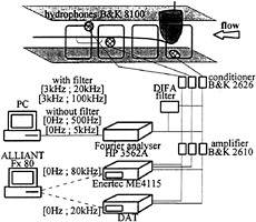
Fig. 5: experimental facility, 1st configuration, acoustic apparatus.
The signal issued from the hydrophone below the tip is conditioned, high pass filtered and amplified. Then the signal is analysed in real time by generation of 4 PSDs of 8000 points on the bandwiths [0 Hz; 500 Hz], [0 Hz; 5 kHz], [3 kHz; 20 kHz] and [3 kHz ; 100 kHz]. On each bandwidth, the Power Spectrum Density or PSD is the result of the mean of 20 analysed signal, except for [0 Hz; 500 Hz] where only 10 were used.
The PSD on [0 Hz; 100 kHz] is deduced from the previous spectral analysis. On each spectrum, the PSD values are averaged on 20 consecutive points which implies 400 points for the PSD. Then, we assemble the PSD values by taking the first spectrum and cutting the second spectrum on 500 Hz up to 5 kHz, the third on 5 kHz up to 20 kHz and the last on 20 kHz up to 100 kHz.
In the second test configuration, a count of noise peaks at the cavitation inception is made. A hydrophone B&K 8104 is flush mounted below the wing tip (Figure 6). A conditioner, a band pass filter [20 kHz; 80 kHz] and a level discrimination are mounted in line before entering in the counter. This
acquisition needs a human intervention to have the best signal to noise ratio and to determine the level of the trigger according to the noise level of the test facility which have been measured during subcavitating phase. The peaks are identified and counted during 10 seconds. Moreover, 2 seconds of acoustic signal were recorded on a mascomp, for more information, with an acquisition frequency of 160 kHz.
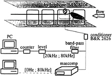
Fig. 6: experimental facility, 2nd configuration, acoustic apparatus.
3.
VISUAL DATA AND CORRELATION
3.1
Cavitation inception
The cavitation inception is first observed on video records, it might be a line of vapor at the center of the vortex, or several transient bubbles captured by the vortex.
As presented in [11], du to the unique fully gas content device of the G.T.H., for water without nuclei injection, the modification of the oxygen content do not affect cavitation inception, provided saturation condition are not reached. For oversaturated flow without injection, σ values at inception are similar to those obtained for low oxygen content and nuclei seeding. For this reason, results were only presented for 30% of oxygen content without nuclei injection, and with two types of bubbles injection called ‘small' and ‘big'.
In Figure 7, the cavitation inception number is ploted as a function of the angle of attack for the three different water qualities. ‘Small' and ‘big' nuclei seeding shift the results towards the small angle of attack. However, the shift is larger for the larger bubbles. Thus, the higher the susceptibility pressure, the easier water cavitates. This phenomenon has to be correlated with visual observations: without nuclei injection, the first cavitation occurence is a vapor tube whereas, with nuclei seeding, nuclei are attracted in the center of the vortex where they grow, explode under the depression, and make the vortex visible.
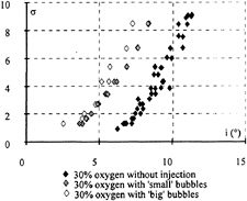
Fig. 7: cavitation inception at V=10 m/s.
The minimum pressure coefficient, Cp(x), in the center of the vortex at the abscissa x is given [8] by:
Cp(x)=–K(x) Cl2 Re0.4 (2)
where K(x) is a coefficient determined experimentally, Cl the lift coefficient and Re the Reynolds number based on the maximum chord length. The lift coefficient is not dependant on the Reynolds number in our experiments, and the slope of the lift coefficient versus the angle of attack equals 0.0598/°.
At inception, the minimum pressure within the vortex, Pmin, can be assumed to be equal to Pv and:
σ=–Cp(x) (3)
If the Reynolds number effects are correctly taken into account by this model, and if Pmin=Pv at inception, a single straight line for each water quality when plotting σ/Re0.4 as a function of Cl2 should be
obtained. As shown in Figure 8, a straight line fits the data for each water quality. Moreover, the slope increases with the ability of the liquid to cavitate (i.e by changing the susceptibility pressure of the freestream nuclei).
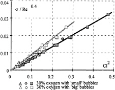
Fig. 8: cavitation inception, triangle: V=15 m/s, diamond: V=10 m/s, square: V=6 m/s.
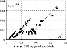
Fig. 9: cavitation inception, triangle: V=15 m/s, diamond: V=10 m/s, square: V=6 m/s.
For water with constant oxygen content and without injection, a strong velocity effect exists (Figure 9). Indeed, by decreasing the freestream velocity from 15 m/s to 6 m/s, for σ/Re0.4=0.01, the incidence angle at inception is increased by a factor of 2. For 6 m/s, we can notice a brake of the line for Cl2<0.6; effectively, in these conditions, the flow is oversaturated and we observe a degassing pnenomenon.
3.2
Correlation of the cavitation inception data
The objective is to obtain a correlation regardless of the water quality and the flow velocity. Using the centerbody venturi VAG, the water quality is characterised by a single parameter, the susceptibility pressure Ps, for a specific nuclei concentration (0.01 nuclei/cm 3). Figure 10 shows the fluid tension Pv-Ps as a function of σ for the ‘small' and the ‘big' bubbles situations. The tension increases with σ for given nuclei injection, and is always significantly larger for the ‘big' bubbles.
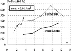
Fig. 10: tension of the liquid versus σ for the nuclei injection used.
According to ([9], [11], [14]) it can be assumed that the cavitation inception occurs at Ps instead of Pv. Hence, the parameter related to the cavitating flow can be expressed by:
(4)
(5)
Using results similar to those presented in Figure 10, a new parameter σ–Δσ is calculated. All the values are now well correlated in the non-dimensional representation (Figure 11), even those without nuclei injection. The main difficulty of this method is the evaluation of Ps. In this case, it is a statistical value, derived from a sample of several litres.
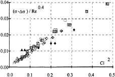
Fig. 11: corrected cavitation parameter at inception versus square lift coefficient, convention for colours and symbols are as previously.
3.3
Developed cavitation
Here, the developed cavitation is characterised by time diameter measurements and estimation of the associated pressure variations.
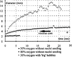
Fig. 12: diameter of cavitating vortex as a flunction of time, σ=4.1, V=10m/s, i=10°.
The time origin is chosen when the cavity is a developed vapor tube without collapsus during time. The radius of the vapour tube at the beginning is smaller than the viscous core diameter of the tip vortex measured by LDV. The diameter varies between 1.5 mm to 15 mm (Figure 12). It increases with time in a way which is very dependent of the water quality. The diameter can be nearly constant for the water with 30% oxygen content without nuclei injection, or increase by a factor 2 on 5 minutes for a water with 80% of oxygen content and no bubbles. For water with injected bubbles, the diameter is multiplied by 4 on the first 5 minutes.
The diameter varies with the flow parameters: the higher the pressure, the thiner the diameter, and the larger the angle of attack, the larger the diameter (Figure 13).
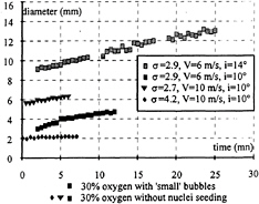
Fig. 13: diameter of cavitating vortex versus time.
Assuming that the growth of the diameter of the vapour tube is due to the diffusion of non condensible gases, the pressure inside the cavity changes with time (from Pv to P(t)). One interesting problem is to estimate this pressure increase which would be responsible for the hysteresis at the desinence cavitation.
In non-cavitating conditions, the tangential velocity of a vortex roll-up, Vt, at the distance r from the center of the vortex, with Euler equations and with a circulation Γ(x) is:
(6)
The depression between two points in the same plane in the flow, at positions r1 and r2, in a steady axisymmetric potential flow, is:
(7)
Now, we apply equation (6) in cavitating conditions. We assume that the circulation is unchanged. At the beginning of the developed vapor tube without collapsus, the radius of the cavity is r0 and the pressure of the cavity is Pv. Between two points, one taken far from the vortex, called ∞, and another taken at the interface of the cavity, the depression is:
(8)
with (1):
(9)
σ0 is the cavitation number of the vapor tube at the beginning.
But the radius of the cavity grows with time. By assumption, this growth is linked to an increase of the pressure inside the vapor tube. At the time t, the cavity has a radius r(t) and a pressure P(t). Then, the depression between a point at the infinity and a point at the interface is:
(10)
But:
P∞–P(t)=P∞–Pv–(P(t)–Pv) (11)
We can define a parameter related to the hysteresis effect, called H, like:
(12)
Then, by substraction of (10) and (9), with (11) and (12):
(13)
Figure 14 shows the variation of H as a function of time, corresponding to the diameters of Figure 12 for water with 30% and 80% of oxygen content. The magnitude of H increases assymptotically with time and depends on the oxygen content: higher oxygen content, higher hysteresis. The slope of the curve at the beginning is high, so, even for two minutes, H>1.
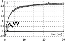
Fig. 14: hysteresis effect during time, same symbols as Figure 12.
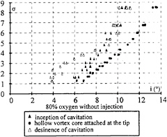
Fig. 15: incipient, attached and desinent cavitation parameter versus angle of attack, V=10 m/s.
Now, we will verify if this order of magnitude is acceptable. In Figure 15, observations of the inception and the desinence cavitation are reported as a function of the angle of attack. The tests were made at constant pressure and varying angle during time. Inception and desinence of cavitation are not at the same angle of attack, which is a consequence of the
hysteresis effect. We underline here that, for equations (6) through (12), we assume a constant circulation. In order to have a constant circulation, we have to provide cavitation tests at constant angle of attack. So, the variation of pressure inside the cavity would be given by the variation of the inlet pressure between the inception and the desinence of cavitation. In Figure 15, if we read the value at a constant angle of attack, for instance at 6°, H equals 2 which is the same order of value as in Figure 14. We notice that we could have directly the value of H if the cavitation tests are performed at constant angle of attack.
4.
ACOUSTIC CHARACTERISTICS
In this part, the acoustic results are presented. We will first discuss about the non-cavitating PSD to characterise the noise of the test facility. Then we will see the influence of the cavity by superimposing the PSDs in non-cavitating and in cavitating conditions. The influence of different parameters like freestream velocity and angle of attack, are shown. The acoustic data are connected to the visual data for better understanding.
4.1
Global behaviour in subcavitating conditions
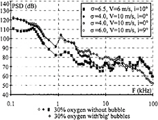
Fig. 16: PSD in subcavitating conditions.
For a given water quality and a given inlet velocity, the acoustic level in subcavitating conditions is independent of the angle of attack and of the pressure level of the test section (Figure 16). The flow velocity affects essentially the bandwidth [100 Hz; 10 kHz] for water without injection: the acoustic level decreases with velocity. At V=10 m/s, the nuclei injection modifies the PSD on the bandwidth [1 kHz; 100 kHz]: the slope is constant, 25 dB/decade, whereas, without injection, the decay of the PSD is of 40 dB on [1 kHz; 10kHz] and rather constant on [10 kHz; 100 kHz]. A specific frequency of the test facility which is 1.25kHz at V=10 m/s, and 0.8 kHz at V=6 m/s can be seen in Figure 16.
4.2
Cavitation inception
A criterion to detect the cavitation inception is the acoustic signal, and particularly the acoustic peaks radiated during the bubble growth when they cavitate. A systematic study was made for a flow with injected nuclei. The collected data are summarised by a count of acoustic peaks for each angle of attack near the angle of the cavitation inception.
Figure 17 shows the peaks during a 10 seconds period as a function of the incidence angle for three cavitation numbers. We obtain a gaussian curve which could be non symmetric. Three characteristic angles of attack can be defined: for the initiation at 1 peak/s, for the maximum count and for the disapearance at 1 peak/s. 1 peak/s corresponds roughly to the visual criterion for cavitation inception in tip vortex.
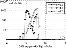
Fig. 17: count of peaks, V=10 m/s.
The acoustic results and the observed data are superimposed in Figure 18. The development of cavitation is added and corresponds to the visual criterion defined as a stable vapor tube attached at the tip of the hydrofoil. The best correlation is observed at 10 m/s: the visual inception corresponds to the first 1 peak/s and the maximum number of peaks is located for the development of cavitation (Figure 18).
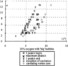
Fig. 18: superimposed of visual and acoustic datas, V=10 m/s.
For σ>4.0, the data at maximum peak/s and 1 peak/s are shifted compared to the visual data. It can be observed that, for these tests, the counts versus the angle of attack are non symmetric and do not extend for unknown reasons over 8° (Figure 17). There is perhaps a problem of level of signal to noise ratio, or the band-pass filter is not adequate for these points. Possibly a more detailed treatment and a best acquisition would give better results.
4.3
Developed cavitation
For water without injection, when cavitation occurs at V=10 m/s, the acoustic level on the bandwidth [500 Hz; 50 kHz] is increased as compared to the subcavitating conditions (Figure 19).
The same phenomena is observed at V=6 m/s on the bandwidth [500 Hz; 20 kHz] (Figure 20). For water with ‘big' bubbles, the bandwidth affected by the increase of the acoustic level is bigger: it begins at 500 Hz and covers the bandwidth until the end (Figure 21).
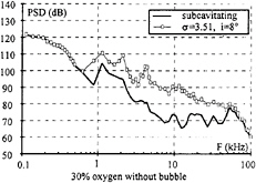
Fig. 19: developed cavitation compared to no-cavitating point, V=10 m/s.
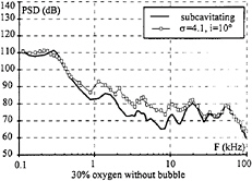
Fig. 20: developed cavitation compared to no-cavitating point, V=6 m/s.
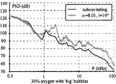
Fig. 21: developed cavitation compared to no-cavitating point, V=10 m/s.
4.4
Frequencies associated to the cavitating vortex core
By comparison of the PSD in subcavitating condition with the PSD in cavitating condition on the bandwidth [0 Hz; 5 kHz], the frequencies, associated to the cavitating conditions were extracted. One or two frequencies are identified by this method for given conditions.
Previous authors, Higuchi et al. [12] and Maines and Arndt [16] for instance, speak about a “singing vortex”. In this phenomenon, “a standing wave develops on the hollow vortex core which radiates significant noise at discrete tone”. In their paper, Maines and Arndt correlate specific frequencies of the singing vortex extracted from acoustic records with the diameter of the cavity.
The possibility to undertake similar analysis on the PSD [0 Hz; 5 kHz] was used. Results such as in Figure 22 were obtained. In this graph, marked lines represent the evolution of the difference between the PDS in non-cavitating and in cavitatin conditions. On each dotted curve, two peaks can be clearly seen: one near 500 Hz and the other near 1.5 kHz and there is no difference of the acoustic signal below 400 Hz. These frequencies vary with the angle of attack.
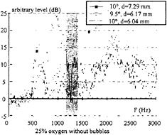
Fig. 22: difference in PSD between non-cavitating and cavitating conditions, the grey region corresponds to the frequencies of the test facility
It can be noticed here a first difference with Maines and Arndt results: two frequencies were obtained for an experimental condition whereas they obtain just one. See for example Figure 23 showing frequencies measured versus a for two velocities (10 m/s and 11 m/s) and two angles of attack (8 deg. and 10 deg.). These measurements were made when the cavity within the tip vortex was attached to the tip of the profil or when the tip of the cavity within the tip vortex begins like a cone-shape in the fluid. Maines and Arndt limit their study to the case of the singing vortex which happens when the cavitating vortex core is attached.
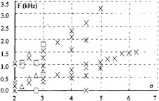
Fig. 23: measured frequencies versus σ value, for two velocities and two angles of attack.
Similar results were observed for a variation of the inlet pressure at constant angle of attack: then the frequencies depend on the inlet pressure. At first order, it seems that frequencies are linked with the diameter of the cavitating vortex core. But, as seen in Figure 22, different informations can be noticed for similar flow conditions and for the same order of diameter: for the diameter d=6.17 mm, we have two identified peaks which do not exist for the diameter d=6.04 mm. This last observation can be related to the problems of reproducibility of the singing vortex encountered by Maines and Arndt.
With the continuous line which corresponds to a measurement made after 15 minutes under constant experimental parameters, a single important peak near 1 kHz appeared. A regular increase of the PSD on [500 Hz; 5k Hz] with the diameter was observed. Unfortunately, the time of existence of the cavitating vortex tube was not systematically acquired during the acoustic measurements. After looking at videos, there is not a distinguishable phenomenon, except perhaps the stability of the tip of the cavity within the
tip vortex. The frequency of 25 Hz of the camera is perhaps not sufficient to analyse the phenomenon. However, the information of the diameter is not sufficient to deduce the frequencies emmitted by the cavity.
4.4
Morozov's model
In the following, we use measured frequencies and associated measured diameter for several cavity within the tip vortex.
A Morozov's model [17] is used where the frequencies are linked to modal deformation of a vapor tube as a function of the mean diameter ‘a'. For a cylindrical cavity within the tip vortex, at constant pressure Pv, the following formulaes can be written:
For m=0:
(14)
with γ is the Euler constant equated to 1.78, F is the frequency, c is the chord length and Vt is the tangential velocity.
For m=1:
(15)
where σ is the cavitation number.
For m=2:
(16)
where T is the surface tension.
Each formula corresponds to a special deformation: when m=0, it is a variation of the diameter; when m=1, it is a sinusoidal deformation of the centerline of the vortex, this phenomenon have to be related to wandering according to Fruman [8]; when m=2+ or 2–, it is an elliptic deformation of the diameter.
In Figure 24, we superimpose the Morozov's frequencies, calculated with the measured diameter, and the measured frequencies. Two possible modes are identified: m=1 and m=2–. It seems that an elliptic deformation and a wandering took place.

Fig. 24: frequencies calculated and measured, the grey region corresponds to the frequencies of the test facility.
In order to enlarge this analysis for all the frequencies measurements, an estimation of the cavitating diamater D was made versus (σ, i and V). For this, as parameters do not vary on a large range, it is assumed that D can be written as:
D=a+bσ+ci+dV (17)
Using size measurements available, parameters a,b,c,d, were identified. D was then calculated for all the test configurations for which peaks were observed and measured in the spectral analysis.
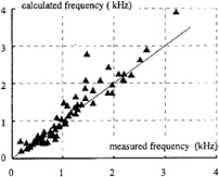
Fig. 25: comparison between calculated and measured frequencies radiated by a developed cavitating vortex.
Figure 25 presents a comparison between frequencies measured in the spectra and frequencies calculated using (15), (16) and (17).
It must be noted that:
-
a good correlation exists between measured and calculated frequencies.
-
the mean error is of 16%, but for 52% of samples the maximum error is lower than 10%, and for 77% of samples the maximum error is lower than 20%.
5.
CONCLUSION
With an hydrofoil of large size, water quality effects on the cavitating vortex was studied. Water was characterised with free nuclei content and oxygen content.
In this experiment, all the data for cavitation inception can be correlated by introducing a cavitation parameter based on the measured susceptibility pressure of the water.
The growth of the cavity within the tip vortex can be explained by diffusive effects linked to the water quality. This leads to understand the hysteris phenomenon at the desinence cavitation. In this analysis, the time must be introduced as an added parameter. Hence, the way the experiments are made is very important for the analysis of the results.
The analysis of the acoustic signal shows that the cavitating vortex radiates frequencies which could be linked to spatial deformation of the cavitating vortex core. In the tests described in this paper, the mode of deformation are m=1 (sinusoidal deformation) and m=2-(elliptic deformation of the diameter). An estimated value, within an error of 20%, of the frequency radiated by the cavity within the tip vortex can be made.
AKNOWLEDGEMENT
The authors wish to thank the Direction des Recherches et de la Technologie (D.R.E.T.), Ministère de la Défense, France, for his financial support.
REFERENCES
1. Abbott I.H., Von Doenhoff A.E., “Theory of wing sections”, Dover publications, 1958
2. Arndt R.E.A., Arakeri V.H., Higuchi H., “Some observation of tip vortex cavitation”, Journal of Fluid Mechanics, 1991, vol 229, pp 269–289
3. Arndt, R.E.A. and Keller, A.P., 1992, “Water Quality Effects on Cavitation Inception in a Trailing Vortex, ” ASME Jour. of Fluids Engineering, Vol. 114.
4. Billet, M.L. and Holl, W.J., 1979, “Scale Effects on Various Types of Limited Cavitation,” Proc. Int. Symp. on Cavitation Inception, ASME Winter Annual Mtg., New York.
5. Briançon-Marjollet L, Fréchou D.; “Cavitation in Le Grand Tunnel Hydrodynamique”, ISPC, China, sept 1992
6. Falcao de Campos J.A.C., George M.F., Mackay M.; “Experimental investigation of tip vortex cavitation for elliptical and rectangular wings”, Cavitation and Multiphase Flow Forum, 1989, ASME FED-vol 79, pp 25–30
7. Fruman D.H., “Recent progress in the understanding and prediction of tip vortex cavitation”, Second International Symposium on cavitation. Tokyo, Japan ( 1994). Proceedings H.Kato ed. pp 19–29
8. Fruman D.H., Dugué C., Pauchet A., Cerrutti, P., Briançon-Marjollet L., “Tip vortex roll-up and cavitation”, 19th Symposium on Naval Hydrodynamics, august 1992, Seoul, Korea
9. Gindroz, B. and Billet, M. 1993, “Influence of the Nuclei on the Cavitation Inception for Different Types of Cavitation on Ship Propelllers,” Cavitation Inception, ASME FED Vol. 177.
10. Godefroy, V., 1994, “Imagerie Numérique Appliquée au Tourbillon Maraginal Cavitant,”, Bassin d'Essais des Carenes, Rep't No. 4.2.97.3649.
11. Gowing S., Briançon-Marjollet L., Fréchou D., Godefroy V., “Dissolved gas and nuclei effects on tip vortex cavitation inception and cavitating core size”, International Symposium on Cavitation, Cav'95, may 1995, Deauville, France
12. Higuchi H., Arndt R.E.A., Rogers M.F., “Characteristics of tip vortex noise”, Journal of Fluids Engineering, december 1989
13. Holl J.W., “An effect of air content on the occurence of cavitation”. Journal of Basic engineering , 1960, pp 941–946.
14. Keller A.P., “Scale effects at beginning cavitation applied to submerges bodies ”. International symposium on cavitation inception 1984.
15. McCormick, “On vortex produced by a vortex trailing edge form a lifting surface ”, Journal of Basic Engineering, sept 1962, pp 369–379 Inception, ASME FED Vol. 177.
16. Maines B.H., Arndt R.E.A., “The case of the singing vortex”, Cavitation and Multiphase Flow, ASME 1995, FED-vol. 21, pp69–74
17. Morozov V.P., “Theoretical analysis of the acoustic emission from cavitation line vortices”. Sov. Phys. Acoust., vol. 19, no 5, 1974 pp 468–471.
DISCUSSION
D.Fruman
ENSTA/GPI, France
The authors have performed a very systematic investigation of tip vortex cavitation inception under various conditions of nuclei seeding. They propose a correction of the incipient cavitation number in order to collapse the data for two seeding conditions (small and large bubbles) in a now classical σc/Re0,4 versus Cp2 plot.
I have 2 types of questions
-
Why has the VAG method not been used to try to correlate also the data for the “no bubbles” situation? Have the measurements of (pc-pu) been conducted? How do the authors explain the very large velocity effects in Figure g?
-
It has been proposed, and used with good success, to obtain the “susceptibility” pressure directly from tip vortex tests (by plotting the difference between the free stream pressure for cavitation inception minus the vapor pressure as a function of the velocity to the power 2,4 for constant incidence angle). Why have the authors not performed these tests and why there is no comparison between theirs and previous methods?
AUTHORS' REPLY
NONE RECEIVED


