Understanding the Contributions of Operations, Technology, and Design to Meeting Highway Capacity Needs (2012)

Below is the uncorrected machine-read text of this chapter, intended to provide our own search engines and external engines with highly rich, chapter-representative searchable text of each book. Because it is UNCORRECTED material, please consider the following text as a useful but insufficient proxy for the authoritative book pages.

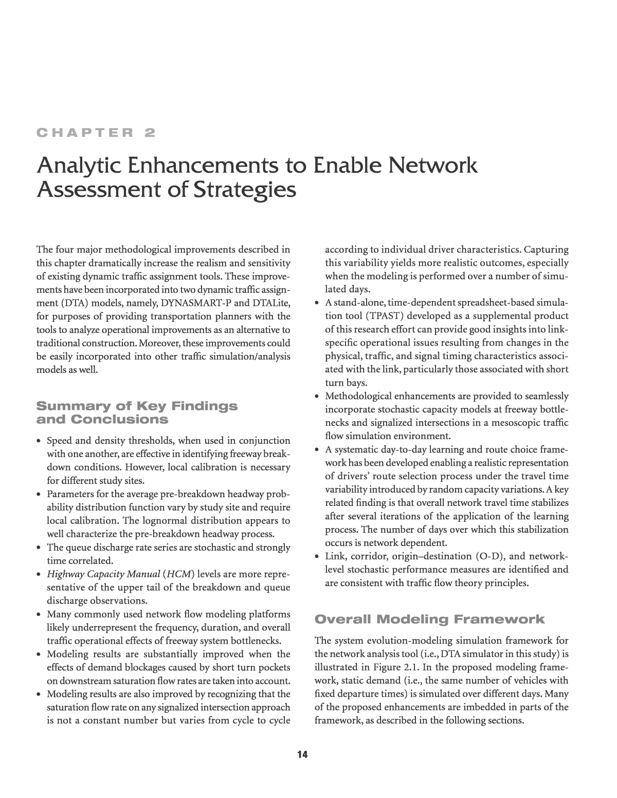
14 C h a p t e r 2 The four major methodological improvements described in this chapter dramatically increase the realism and sensitivity of existing dynamic traffic assignment tools. These improve- ments have been incorporated into two dynamic traffic assign- ment (DTA) models, namely, DYNASMART-P and DTALite, for purposes of providing transportation planners with the tools to analyze operational improvements as an alternative to traditional construction. Moreover, these improvements could be easily incorporated into other traffic simulation/analysis models as well. Summary of Key Findings and Conclusions • Speed and density thresholds, when used in conjunction with one another, are effective in identifying freeway break- down conditions. However, local calibration is necessary for different study sites. • Parameters for the average pre-breakdown headway prob- ability distribution function vary by study site and require local calibration. The lognormal distribution appears to well characterize the pre-breakdown headway process. • The queue discharge rate series are stochastic and strongly time correlated. • Highway Capacity Manual (HCM) levels are more repre- sentative of the upper tail of the breakdown and queue discharge observations. • Many commonly used network flow modeling platforms likely underrepresent the frequency, duration, and overall traffic operational effects of freeway system bottlenecks. • Modeling results are substantially improved when the effects of demand blockages caused by short turn pockets on downstream saturation flow rates are taken into account. • Modeling results are also improved by recognizing that the saturation flow rate on any signalized intersection approach is not a constant number but varies from cycle to cycle according to individual driver characteristics. Capturing this variability yields more realistic outcomes, especially when the modeling is performed over a number of simu- lated days. • A stand-alone, time-dependent spreadsheet-based simula- tion tool (TPAST) developed as a supplemental product of this research effort can provide good insights into link- specific operational issues resulting from changes in the physical, traffic, and signal timing characteristics associ- ated with the link, particularly those associated with short turn bays. • Methodological enhancements are provided to seamlessly incorporate stochastic capacity models at freeway bottle- necks and signalized intersections in a mesoscopic traffic flow simulation environment. • A systematic day-to-day learning and route choice frame- work has been developed enabling a realistic representation of drivers’ route selection process under the travel time variability introduced by random capacity variations. A key related finding is that overall network travel time stabilizes after several iterations of the application of the learning process. The number of days over which this stabilization occurs is network dependent. • Link, corridor, origin–destination (O-D), and network- level stochastic performance measures are identified and are consistent with traffic flow theory principles. Overall Modeling Framework The system evolution-modeling simulation framework for the network analysis tool (i.e., DTA simulator in this study) is illustrated in Figure 2.1. In the proposed modeling frame- work, static demand (i.e., the same number of vehicles with fixed departure times) is simulated over different days. Many of the proposed enhancements are imbedded in parts of the framework, as described in the following sections. Analytic Enhancements to Enable Network Assessment of Strategies

15 Note: DTA = dynamic traffic assignment; MOE = measure of effectiveness. 9. Update Mean Travel Time from day d-K to day d 8. Triggering Mechanism Habitual Path Switching 11. Habitual Path Updating Day d++ Stochastic Link Performance and Breakdown Probability Database 10. Post-Trip Alternative Route Generation Day-to-day Learning Traffic MOE Database Internal Data InterfaceAlgorithmic ModuleInput Parameters D. % of Travelers Willing to Learn DTA Simulator No 7. Dynamic Mesoscopic Traffic Simulator Updated Path Flow Pattern 12. Stability Checking Experienced Travel Time on Day d for Each Vehicle 3. Stochastic capacity generation on arterial links 2. Stochastic capacity generation on freeway bottlenecks 6. Bounded Rationality Rule for Within-day Route Switching A. Merge/ Diverge/Weaving Bottleneck Locations 1. Bottleneck Identification 4. Pre-trip/En-route Path Generation 5. Vehicle Loading with Habitual Path B. Market Penetration Rates of Traveler Information Users C. Parameters of Bounded Rationality Rule for Within-day Path Switching E. Parameters of Bounded Rationality Rule for Habitual Path Switching Figure 2.1. Comprehensive conceptual simulation framework. The following three critical inputs (illustrated in Figure 2.1) should be prespecified by users: • Time-dependent traffic demand; • Bottleneck locations; • Percentages of unequipped, pretrip, and en route users; and • Parameters of the bounded rationality rule. Figure 2.1 demonstrates the entire conceptual simula- tion framework implemented in DYNASMART-P. Two key components, stochastic capacity generation on freeway bottlenecks and signalized arterial and route choice mecha- nism, are not illustrated in detail; because of their signifi- cance, they are discussed in depth in the following sections of this chapter. There are four major enhancements: 1. Stochastic capacity for freeway bottlenecks and capacity allocation at freeway merge areas; 2. Stochastic capacity and turn pocket analysis on arterials; 3. Implementation of a day-to-day learning paradigm; and 4. New performance measures and implementation.

16 enhancement 1: Stochastic Capacity for Freeway Bottlenecks In this section, the stochastic nature of freeway breakdown and queue discharge is discussed through a comprehensive analysis of sensor data collected at bottleneck sites in the San Francisco Bay Area, California, and San Antonio, Texas. A new procedure is proposed to define the stochasticity of freeway breakdown and queue discharge based on time-indexed data of speed-flow profiles (1). Stochastic Breakdown Characteristics In the 2000 edition of the Highway Capacity Manual, freeway capacity is defined as “the maximum hourly rate at which vehi- cles reasonably can be expected to traverse a point or a uniform section of a roadway during a given time period under prevail- ing roadway, traffic, and control conditions” (2). In keeping with the definition of conventional freeway capacity, it is widely accepted by most traffic analysts that the facility will experi- ence breakdown (i.e., a transition from an uncongested state to a congested state) only if the traffic demand exceeds a spec- ified capacity value. Therefore, when freeway capacity is taken to be a constant value, breakdown is treated as a deterministic phenomenon. However, an emerging body of research (3–8) indicates that traffic flow rate during the time intervals pre- ceding observed instances of freeway breakdown (called pre-breakdown flow rate in this study) is better represented as a random variable than a fixed value. Zurlinden (9) and Brilon (10) developed a methodology to derive roadway pre- breakdown distribution functions for the purpose of imple- menting this stochastic capacity concept. In the most recent study, Brilon (11) suggested the Weibull distribution for charac- terizing stochastic capacity based on traffic data from Germany. Based on the probabilistic nature of freeway capacity, Dong and Mahmassani (12) first illustrated the significant effects of the stochastic concept on the study of travel time reliability. The conventional definition of fixed capacity for uninter- rupted flow facilities has the practical drawback of under- representing the frequency, duration, and therefore traffic operational impact of freeway system bottlenecks. In order to quantify accurately the capacity benefits of operations, design, and technology improvements, it is necessary to develop realis- tic, implementable capacity models for freeway operations. The following sections provide details of the procedure followed to develop the stochastic pre-breakdown headway distribution for freeway bottlenecks implemented in DYNASMART-P. Identifying Freeway Bottlenecks As a basis for developing and validating stochastic freeway bottleneck models, the most common freeway bottleneck fea- ture, on-ramp junctions, was selected for detailed study. Data were assembled from the TransGuide system (13) in San Antonio and from PeMS data (14) archived for the San Francisco Bay Area (Caltrans District 4). Data for both loca- tions are readily available from online databases. The TransGuide database provides traffic volume, speed, and occupancy data gathered from the initial 26 miles of instru- mented highways within the Texas Department of Transporta- tion TransGuide project. The extracted data set for this study is the daily raw data (20-second intervals) from 01/01/2007 to 09/30/2008. The TransGuide data include a small number of missing observations which required removal of a small portion of data from the aggregated set. The Bay Area data used in this study are processed traffic data, which include volume, speed, and occupancy. The data cover the period from 01/01/2007 to 09/30/2008 and are aggregated at 5-minute intervals. Since the Bay Area data are already preprocessed and aggregated, the missing observations have been estimated in the data set. Both TransGuide and PeMS databases provide detailed location information for each sensor on the freeway system. As discussed below, these data were important for selecting appropriate bottleneck locations for this study. The informa- tion from the TransGuide and PeMS databases is summarized in Appendix A. The PeMS system identifies active bottleneck locations for the Bay Area; those that experience congestion for more than 10 days per month were selected for study. In contrast, the TransGuide database does not identify active bottlenecks in the freeway network. Therefore, geometric bottlenecks were identified through visual inspection by using Google Maps of the areas covered by TransGuide detectors. To control for possible confounding operational effects and to isolate ramp merge bottleneck effects, a systematic process was developed for study site selection. Suitable bottleneck sites met the fol- lowing three criteria: 1. Sufficient distance between the on-ramp and the nearest downstream bottleneck. The longer the distance to a poten- tial downstream bottleneck (e.g., on-ramp or off-ramp), the greater the likelihood that the data are not confounded by the presence of downstream queues regularly spilling back to the bottleneck location under consideration. 2. Suitably placed sensor data. An ideal detector is just down- stream of the corresponding bottleneck. 3. Presence of traffic demand high enough to yield regular freeway breakdown. This criterion ensures an adequate sample size. Because the candidate sites in the Bay Area are active bottle- necks, the third criterion was not a significant factor for the PeMS data. In the San Antonio area, however, traffic data were retrieved from the TransGuide system to evaluate the third criterion for sites that met the first and second criteria.

17 Based on the three criteria, seven on-ramp bottlenecks (three with three travel lanes and four with four travel lanes) were selected as the study sample. Two of the sites are in the San Antonio area, and the remaining five are in the Bay Area. The basic information about each site is summarized in Table 2.1. As mentioned above, the data in the Bay Area are aggre- gated into 5-minute intervals and the San Antonio data into 20-second intervals. Consistent with HCM 2000, both data sets were aggregated into 15-minute intervals prior to analysis. Method for Implementing Stochastic Capacity A critical step in developing pre-breakdown headway dis- tributions is determining when breakdown occurred on the basis of a review of historical speed-flow data. The pub- lished studies specified a critical speed or a critical speed drop to define the freeway breakdown. However, while such a speed-based threshold can be well defined in reference to representative traffic flow characteristics, its value will vary by location. For example, extensive analysis of data from Los Angeles freeways suggests that free-flow speed is around 60 mph and that at breakdown the operating speed rapidly drops below 40 mph (15). Researchers in Los Angeles there- fore specified a minimum speed differential of 20 mph and a speed threshold of 40 mph to identify a breakdown event by using 5-minute data. Using data obtained from Toronto freeways, on the other hand, Elefteriadou (16) defined that breakdown occurred “when the average speed of all lanes on the freeway dropped below 90 km/hr (56 mph) for a period of at least five minutes.” These examples demonstrate that breakdown events are unique to local conditions and that use of a specific, universal speed threshold is not advis- able. Freeway breakdown events should be defined on the basis of speed thresholds extracted from local speed-flow observations. Moreover, as discussed later in this chapter, it is problematic to use speed as the only criterion to define breakdown. Breakdown determination is the critical starting point for both stochastic capacity and queue discharge studies. As mentioned earlier, although most previous studies used speed as the threshold, a single speed threshold was not considered appropriate for determining congested conditions based on the speed-flow relationships observed in field data. Figure 2.2 shows 21 months of 15-minute freeway data from I-880 in the Bay Area. The horizontal line superimposed on the plot indicates the speed boundary that was used to isolate con- gested conditions. As is apparent from the graph, a single speed threshold is not sufficient for determining congested conditions. Observed conditions exhibiting a flow rate lower than 1,000 vehicles per hour per lane but with speeds higher than 40 mph were considered to be reflective of anomalous free-flow conditions rather than congested conditions. The data pattern shown in Figure 2.2 is typical of the seven on- ramp sites, and the presence of low-flow observations below the critical speed threshold creates the need for a robust phase boundary for defining congested conditions. A combination speed and density threshold (diagonal line in Figure 2.2) was applied to identify congested conditions, thereby avoiding the inclusion of anomalous low-speed data. Traffic states are considered to represent congested condi- tions only when • The observed speed is below the critical speed. • The observed density is greater than or equal to the bound- ary between levels of service C and D (LOS C/D). As mentioned above, the critical speed and the density at the LOS C/D boundary [e.g., in HCM 2000, 26 passenger cars per mile per lane (pc/mi/lane) is the boundary that separates LOS C from LOS D] are locally calibrated for each Table 2.1. Basic Information about the Study Sites Site Number Highway Direction Number of Lanes Distance to Downstream Bottleneck (km) Distance to Detector (km) 1 I-880 (BA) S 4 3.0 0.1 2 I-680 (BA) S 3 2.6 0.1 3 I-280 (BA) N 4 NA 0.36 4 I-580 (BA) W 4 NA 0.25 5 I-680 (BA) N 4 6.1 0.12 6 I-35 (SAT) N 3 3.6 0.18 7 I-35 (SAT) S 3 2.2 0.38 Note: NA indicates that the distance to downstream bottleneck is very long (more than 10 km). BA = Bay Area; SAT = San Antonio.

18 of the specific study sites. The procedure for calculating these site-specific thresholds is described in the following paragraphs. First, 15-minute flow rate values in the top 1 percentile tail are identified. The average of this sample of near maximum flows was generally equivalent to the traditional capacity defined in the HCM. The density for each 15-minute obser- vation is then calculated as shown by Equation 2.1: (2.1)k q = µ where k = density for each 15-minute observation (veh/mi/lane), q = 15-minute flow rate for the top 1 percentile flows (veh/h/ lane), and µ– = space mean speed (mph) The critical speed is then calculated as shown in Equation 2.2: (2.2) q kcritical ∑ ∑µ = where q = 15-minute flow rates in the top one percentile flows and k = 15-minute density values corresponding to the top 1 percentile flows. The equivalent density at capacity based on HCM defini- tion is calculated by Equation 2.3: 1 (2.3)k n kcapacity ∑= where n = number of 15-minute observations in the top 1 percentile flow region. Finally, the adjusted HCM-based critical density threshold (LOS C/D boundary) is calculated by Equation 2.4: 26 45 (2.4)k k critical capacity( ) = where 26 pc/mi/lane represents the maximum density per lane passenger car equivalent density for LOS C for basic free- way segments per HCM 2000 and 45 pc/mi/lane represents the corresponding per lane passenger car density at capacity. Equation 2.4 provides adjusted values for the LOS C/D thresholds based on the observed density at capacity. In sum- mary, traffic conditions observations are identified as repre- senting congested flow when the observed 15-minute speed is less than the critical speed and the observed 15-minute density is greater than the critical density. Each study site was analyzed independently. Speed and vehicle count data were summarized in 15-minute intervals across all lanes. The vehicle count data were then expressed as equivalent hourly flow rates per lane. The traffic parameters for each site are summarized in Table 2.2. Breakdown from Free-Flow Conditions In deterministic traffic models, such as that of the HCM, there are two basic traffic states in uninterrupted freeway operation: uncongested and congested flow. In defining stochastic capacity, the focus lies on the pre-breakdown state (i.e., the uncongested states just preceding the breakdown state). The breakdown state is the first in what may be a series of congested state observations. Once the breakdown states were identified, all the corresponding pre-breakdown states were selected from each data set. For purposes of implemen- tation in the mesoscopic model, DYNASMART-P, the pre- breakdown flow rates were first converted into passenger car Note: veh/h/ln = vehicles per hour per lane. 0 10 20 30 40 50 60 70 80 90 100 0 500 1000 1500 2000 2500 15 min Flow Rate (veh/h/ln) Sp ee d (m ph ) Figure 2.2. I-880 speed-flow data. Table 2.2. Calibrated Traffic Parameters for Each Study Site Site Number Highway Average Top 1 Percentile Flow Rate (veh/h/lane) Critical Speed (mph) Density (C/D) (veh/mi/lane) 1 I-880 (BA) 2,052 56 21 2 I-680 (BA) 2,093 53 23 3 I-280 (BA) 2,183 53 24 4 I-580 (BA) 1,982 49 23 5 I-680 (BA) 2,127 54 23 6 I-35 (SAT) 1,992 47 23 7 I-35 (SAT) 2,172 63 20

19 equivalent flows and then aggregated into 15-minute pre- breakdown headways (i.e., 3,600/flow rate). Heavy vehicle count data were not available for the sites in this study. There- fore, the HCM 2000 default of 5% heavy vehicles and the pas- senger car equivalent for trucks and buses of 1.5 for a level general segment was used to convert the TransGuide and PeMS data to passenger car equivalent flow rates. It is desirable to exclude pre-breakdown flow rate under nonrecurring conditions as much as possible. However, in the absence of incident logs, a statistical approach was applied to exclude outlying pre-breakdown flow rates. As shown in Equation 2.5, a pre-breakdown flow rate is identified as an outlier if: 1.5 or 1.5 (2.5)0.25 0.75q Q IQR q Q IQR< − > + where Q0.75 = 75th percentile flow rate (pc/h/lane), Q0.25 = 25th percentile flow rate (pc/h/lane), and IQR = Q0.75 - Q0.25. The speed-flow diagram in Figure 2.3 shows the pre- breakdown and outlier observations for one study site (I-880). Almost all flow rates below the HCM equivalent LOS C/D den- sity boundary were identified as outliers. For the 15-minute aggregated traffic data, it is reasonable that the pre-breakdown flow rates would not occur at LOS C or better under the prevailing roadway, traffic, and control conditions. Statistical tests were conducted to determine the probabil- ity distributions that reflect the stochastic characteristics of freeway pre-breakdown headway. The most common tests for goodness of fit are the Kolmogorov–Smirnov (K-S) test, chi- square test, and Anderson–Darling (A-D) test. All are used to decide whether a data sample belongs to a population with a specific distribution. A chi-square test could be applied to test any univariate distribution; however, the values of the chi- square statistic are quite sensitive to how the data are binned (17). The Anderson–Darling statistic is a measure of how far the data points lie from the fitted distribution. However, the A-D test is not a distribution-free test. The critical values for the A-D test must be calculated for each distribution, and they are only available for a very limited number of dis- tributions (18). The K-S statistic also quantifies a distance between the empirical distribution function of the sample and the cumulative distribution function of the reference dis- tribution. The K-S test is distribution-free in the sense that it makes no assumption about the underlying distribution of data (19). Another advantage of the K-S test is that it is an exact test, while the chi-square goodness-of-fit test depends on an adequate sample size for the approximations to be valid (17). Therefore, the K-S test was applied here to examine which distribution functions provide the best fit to the pre- breakdown headways. The shifted lognormal, normal, exponential, Weibull, and gamma distributions were evaluated for fit with the field data. For each of these, a K-S statistic was calculated. As indicated in Table 2.3, the shifted lognormal distribution yields the lowest K-S statistic values across all study sites. Figure 2.4 illustrates a sample pre-breakdown headway distribution for one study site on I-880 in the Bay Area. As shown in the figure, a single headway value is not appropriate for defining breakdown on freeways. The trend illustrated 0 10 20 30 40 50 60 70 80 90 100 0 500 1000 1500 2000 2500 Sp ee d (m ph ) 15 min Flow Rate (pc/h/ln) Pre-Breakdown Outliers Critical Speed LOS C/D Figure 2.3. Pre-breakdown flows and outliers for I-880.

20 also indicates that the slope continually decreases with increas- ing values of time headway (i.e., decreasing flow rate). This trend is consistent with findings from previous studies (7, 11) showing that the probability of breakdown increases with increasing flow rate. The figure also gives the corresponding 15th, 50th, and 85th percentile flow rates derived from the dis- tribution. For example, if capacity is defined as a 15-minute flow rate that is sustainable 85% of the time, the corresponding capacity value could be 1,778 pc/h/lane. Similar to the site-specific process for identifying break- down observations, a local pre-breakdown headway distribu- tion was estimated independently for each on-ramp site. The distribution parameters for the seven sites are summarized in Table 2.4. Although the distribution parameters varied among study sites, it was found that the pre-breakdown headways of all seven sites are best modeled as a shifted lognormal random variable. The average shift at the seven study sites is 1.519 sec- onds (standard deviation of 0.053 seconds), which is equiva- lent to 2,370 pc/h/lane. This value is very close to value of predicted HCM 2000 capacity. The mean pre-breakdown headway at the seven study sites is 1.886 seconds (standard deviation of 0.094 seconds), which is equivalent to 1,909 pc/h/ lane. The scale parameters vary among different sites and may depend on the specific characteristics of the analyzed freeway section, local differences in driver behavior, pre- vailing weather conditions, and other factors. In order to implement the stochastic capacity in DYNASMART-P and then test the effects of stochastic free- way capacity on SSRs and network performance, a single shifted lognormal distribution was proposed by aggregating all the pre-breakdown headway observations in the above Table 2.3. Computed Kolmogorov–Smirnov (K-S) Statistic Values by Distribution Tested Distribution Site Number 1 2 3 4 5 6 7 Shifted lognormal 0.039 0.074 0.032 0.066 0.022 0.094 0.058 Normal 0.140 0.132 0.128 0.168 0.072 0.226 0.120 Exponential 0.239 0.333 0.226 0.227 0.296 0.189 0.133 Weibull 0.385 0.410 0.380 0.390 0.230 0.310 0.170 Gamma 0.128 0.122 0.119 0.156 0.063 0.209 0.106 0.00% 10.00% 20.00% 30.00% 40.00% 50.00% 60.00% 70.00% 80.00% 90.00% 100.00% 0 50 100 150 200 250 300 Fr eq ue nc y Time Headway (s) 15th Flow =2114 pc/h/ln Frequency Fitted_Log-Normal Cumulative % Fitted_Cumulative 85th Flow =1778 pc/h/ln 50th Flow =1976 pc/h/ln Figure 2.4. Pre-breakdown headway distribution for I-880.

21 seven study sites. The corresponding parameters are shift = 1.5 seconds, µ = -0.97, and s = 0.68. It should be noted that if the point of interest is a single on-ramp bottleneck, as stated before, local calibration is recommended to develop the average pre-breakdown headway distribution model. For a relatively large network, however, a single set of parameters for the pre-breakdown model developed from the data avail- able is efficient for model implementation and should be accurate enough for the network-level analysis. Recovery from Breakdown Conditions Similar to the conventional definition of capacity in the HCM, the queue discharge flow rate is also typically char- acterized in a deterministic manner. In other words, after a breakdown occurs, the queue will discharge at a constant flow rate. Based on field data, Lorenz and Elefteriadou (7) have clearly demonstrated that the queue discharge flow rate is also stochastic in nature. In a recent study, Dong and Mahmassani (20) suggested a linear relationship between queue discharge rate and the pre-breakdown flow rate. How- ever, the studies for the queue discharge behaviors, especially the stochastic characteristics, are quite limited. In this sec- tion, queue discharge behaviors under the stochastic capacity scenario were discussed. Considering the stochastic nature of freeway capacity, it is quite possible that the queue discharge flow rate is correlated with the stochastic pre-breakdown flow rate preceding the queue existence. In addition, the 15-minute field data have shown that the queue could be discharged over multiple time intervals. By examining the observational data, it was found that the queue discharge rate could be updated with stochastic time-correlated recursions. A simple first-order auto regressive model is proposed as follows in Equation 2.6: 1 (2.6)1C C tt t t ( )= α + µ + ε ≥− where Ct = queue discharge rate at time interval t in pc/h/lane, a = coefficient, µ = intercept, and et~N(0, s2) = random error. When t = 1, C0 is the pre-breakdown flow rate. If we assume b = 1 - a, then the first two terms of the model above can be rewritten as shown in Equation 2.7: 1 (2.7)1 1C C C tt t c t( ) ( )= + β µ − ≥− − where b = a linear parameter that models the strength of regression to the mean and µc = the average discharge rate in pc/h/lane. For the DYNASMART-P model implementation, a ran- dom error term is added based on the error distribution of the fitted model. As shown in Equation 2.8, stochastic inno- vation term et ~ N(0, s2) is proposed. Therefore, the recursive model to update the queue discharge rate (per lane) is 1 (2.8)1 1C C C tt t c t t( ) ( )= + β µ − + ε ≥− − The traffic data from the study site on I-880 in the Bay Area were used to fit the proposed queue discharge model. The fitting procedure began with the series only having two time intervals (i.e., pre-breakdown time interval and queue discharge interval). The duration of the queue discharge interval begins with one time interval and then is continu- ously extended by a time interval if queues are still present at the end of the time interval. Table A.3 in Appendix A shows fitted parameters for the various cumulative queue duration Table 2.4. Summary of Pre-breakdown Headway Distribution Parameters Site Area Lognormal Parameter Maximum Pre-breakdown Flow (pc/h/lane) Mean Pre-breakdown Flow (pc/h/lane)Shift (s)  s 1 I-880 (BA) 1.536 -1.255 0.520 2,343 1,933 2 I-680 (BA) 1.486 -1.139 0.288 2,422 1,978 3 I-280 (BA) 1.626 -1.297 0.516 2,214 1,857 4 I-580 (BA) 1.489 -1.537 0.488 2,418 2,079 5 I-680 (BA) 1.527 -0.730 0.255 2,358 1,778 6 I-35 (SAT) 1.499 -1.147 0.689 2,371 1,893 7 I-35 (SAT) 1.470 -1.021 0.678 2,449 1,871

22 lengths. The results indicate that there is a statistically sig- nificant relationship between Ct and Ct-1. The relatively high R2 value also suggests that the proposed model matches the data very well. At least 73% (the minimum R2 value in Appendix A) of the variation in the response variable Ct, can be explained by the proposed model. Moreover, by using an average discharge rate of 1,850 pc/h/lane and b as 0.2 for all the queue duration lengths, a simple overall queue discharge model could be generated with few impacts on the goodness of fit of each subgroup. Based on the model fitting results, a stochastic innovation term et ~ N(0, s2) is also proposed with s = 100 pc/h/lane. Figure 2.5 illustrates the proposed simplified recursive queue discharge model. In summary, the queue discharge model is based on all break- down flow observations with three primary char acteristics: • The queue discharge rate series are strongly time correlated. • The queue discharge rates have a stochastic, random inno- vation component. • The queue discharge rates converge to the mean discharge rate for breakdowns that are initiated with stochastic capac- ities that are in the tails of the pre-breakdown headway distribution. Supplemental Freeway Capacity Enhancement: Capacity and Queue Allocation at Merge Points When two traffic streams merge and the sum of their demand is greater than the capacity of the downstream roadway, traffic queues will be generated on the upstream links. How and where queues grow and dissipate at the merge point fully depends on how the available downstream capacity is allocated to the entering traffic streams. Following a comprehensive literature review, the research team developed a series of algorithms to allocate capacity at merge points. Basically, the proposed capac- ity allocation algorithms focused on two scenarios: freeway-to- freeway merge and on-ramp-to-freeway merge. Freeway-to-Freeway Merge The proposed allocation algorithm for freeway-to-freeway merge is relatively simple: the allocated capacities for the enter- ing freeway streams are proportional to the incoming upstream flow rates. For example, if the capacity of the downstream freeway link is 3,600 passenger cars per hour (pcph) and the entering flow rates of the two upstream freeway links are 2,800 pcph (Freeway 1) and 1,400 pcph (Freeway 2), the allocated capacity for Freeway 1 is 2,400 pcph (i.e., 3,600 • 2/3) and for Freeway 2 is 1,200 pcph (i.e., 3,600 • 1/3). Therefore, the queue growth rates for Freeway 1 and Freeway 2 would be 400 pcph and 200 pcph, respectively, assuming no changes in demand. on-raMp-to-Freeway Merge Compared with the freeway-to-freeway merge, the proposed allocation algorithm for on-ramp-to-freeway merge is rela- tively complex, because the freeway mainline flow has higher priority than that of the on-ramp. Therefore, the basic con- cept is to apply the capacity allocation according to the rela- tive demand distribution between the two entering traffic streams. Based on the possible demand combinations, five demand regions have been defined. The capacity allocation process varies by region. As shown in Figure 2.6, the x-axis 500 700 900 1100 1300 1500 1700 1900 2100 2300 2500 500 1000 1500 2000 2500 C( t) C(t-1) Figure 2.5. Simplified recursive queue discharge model.

23 represents the on-ramp demand and allocated capacity, while the y-axis represents the total freeway mainline demand and allocated capacity. The diagonal line represents the merge area—or downstream freeway—capacity (no served flows can be above that line); the two vertical lines represent the ramp roadway capacity (Line A), and 50% of the freeway rightmost lane capacity (Line B). All the dashed lines repre- sent the region boundaries. Regions I through V depict the areas with various combinations of ramp and freeway mainline demands. It should be noted that Region V is below the diago- nal line, which represents demand flows that are below the downstream capacity and therefore there is no effective queuing on either stream in this region and both ramp and mainline demand are fully served. Regions I–IV are defined on the basis of relative demand distribution as follows. In all the following cases, demand exceeds that of Region V, that is DF + DR > Downstream Capacity Region I: DF < CRamp; Region II: CRamp < DF < C - 0.5CRM; Region III: C - 0.5CRM < DF & DR > 0.5CRM; Region IV: C - 0.5CRM < DF & DR < 0.5CRM. where DF = freeway demand (vph), DR = on-ramp demand (vph), C = capacity at merge point (vph), CRamp = on-ramp roadway capacity (vph), and CRM = freeway rightmost lane capacity (vph). The following sections explain the basis for allocation of available downstream capacity in each region. Region I In this region, the freeway mainline demand can be fully served with the available downstream capacity. However, the on-ramp demand is greater than the on-ramp capacity, and therefore, the actual entering on-ramp flow rate at the merge point is at the on-ramp capacity value. In Figure 2.7, the point (DF, DR) represents a certain demand combination and the horizontal line demonstrates how the capacity at the merge point is allocated to both the freeway and on-ramp. CF and CR represent the allocated capacities for the freeway and on- ramp, respectively. In this region, no queue will be observed on either the freeway or the on-ramp links. Since the on- ramp demand is greater than the on-ramp capacity, queuing is expected to occur upstream of the on-ramp. The capacity at the merge point is also not fully used (Point C is below the downstream capacity line). Region II In Region II, the capacity of merge point is fully used and is allocated to the two incoming streams as shown in Figure 2.8. Therefore, in this region, there is no queuing on the free- way mainline and queues occur exclusively on the on-ramp link. The rate of queuing at the merge point will be CRamp - CR On-Ramp Demand & Capacity Downstream Capacity M a in li n e F re e w a y D e m a n d & C a p a ci ty IV V III III II I II B A Ramp Capacity½ Rightmost Lane Capacity Figure 2.6. Demand regions for on-ramp-to-freeway merge.

24 vehicles per hour and upstream of the on-ramp roadway at a rate of DR - CRamp vehicles per hour. Region III In Region III, the ramp demand exceeds one half the capacity of the freeway mainline, as shown in Figure 2.9. In this region, a single capacity allocation point (CR - CF) is recommended to allocate the available downstream capacity. Therefore, for all demand combinations in this region, the merge capacity allocated to the on-ramp traffic is exactly half of the freeway rightmost lane capacity (i.e., 0.5CRM), and freeway traffic will consume the remaining downstream capacity (i.e., C - 0.5CRM). It should be noted that in Region III, queues will occur on both the freeway mainline and the on-ramp. The rate of queuing on the ramp is at a rate of DR - 0.5CRM vehicles per hour, if DR < CRamp, or at rate of CRamp - 0.5CRM vehicles per hour, if DR < CRamp; and on the freeway mainline at the rate of DF - CF vehicles per hour. Region IV In Region IV, the on-ramp demand is relatively low. The capacity at the merge point will be allocated as shown in Figure 2.10. Therefore, in this region, there is no queuing on the on-ramp and queues are exclusively allocated to the freeway mainline, and will occur at the rate of DF - CF vehicles per hour. IV C CR (DRDF) DR (CFDF) III III IIII On-Ramp Demand & Capacity M a in li n e F re e w a y D e m a n d & C a p a ci ty I Ramp Capacity½ Rightmost Lane Capacity Figure 2.7. Capacity allocation for demand in Region I. IV C CR (DRDF) DR (CFDF) III III IIII On-Ramp Demand & Capacity M a in li n e F re e w a y D e m a n d & C a p a ci ty I Ramp Capacity½ Rightmost Lane Capacity Figure 2.8. Capacity allocation for demand in Region II.

25 enhancement 2: Stochastic Capacity and turn pocket analysis on arterials Traffic flow along arterial street systems is affected by the operating characteristics of each individual approach along the arterial and system effects from upstream and down- stream intersections (i.e., queue spillback or blockage). A significant body of knowledge is available in the Highway Capacity Manual (2000) for estimating capacity at individ- ual approaches based on a number of factors including lane geometry, lane widths, signal timing, and turning movement demand. However, one of the traditional shortcomings of arte- rial analysis procedures is the lack of ability to model system effects, particularly in the context of a network and short of developing resource-intensive microsimulation models. The advancement of DTA models such as those applied in this research effort allows for the analysis of system-level effects that incorporate the unique factors of individual intersection approaches along with upstream and downstream conditions for each approach. In order to improve the realism of operating conditions along arterials, two significant enhancements were made to the DTA models used in this research project to test the effects of non-lane-widening strategies: 1. Stochastic capacity for arterials. The bottleneck points for signalized arterials are most often located at intersections. Ramp Capacity½ Rightmost Lane Capacity IV (D D )R F DF (C D )R F III III IIII On-Ramp Demand & Capacity M a in li n e F re e w a y D e m a n d & C a p a ci ty I DR Figure 2.9. Capacity allocation for demand in Region III. Ramp Capacity IV C (D D )R F (C D )R R III III IIII On-Ramp Demand & Capacity M a in li n e F re e w a y D e m a n d & C a p a ci ty I DF CF ½ Rightmost Lane Capacity Figure 2.10. Capacity allocation for demand in Region IV.

26 Traditional DTA models assume a constant saturation flow rate during the green time for either the approaching links or for individual turn movements at these locations. How­ ever, it is well known that the saturation flow rate for indi­ vidual links and turn movements varies significantly according to the behavior of individual drivers. At signalized intersections this is revealed by saturation flow rates that vary from cycle to cycle. Therefore, a stochastic approach was developed that allows the capacity of a signalized inter­ section to vary during each time interval (typically 15 min­ utes) according to an empirically observed distribution. 2. Short turn pocket effects. The approaches to signalized inter­ sections along arterial roadways often include left and right turn pockets as a way of separating turn movements and increasing capacity. But when the queue length of through and/or turning vehicles extends beyond the length of the turn pocket, the result is a demand blockage that prevents upstream vehicles from taking advantage of the capacity that is available at the intersection. This is an important phenom­ enon to model in oversaturated networks because it directly affects the efficiency and productivity (or SSRs) of individ­ ual links and turn movements. Therefore, an enhanced model was developed that recognizes when queue lengths exceed available storage lengths at these locations and then adjusts the downstream discharge rate accordingly. The following sections describe the enhancements made to the DTA models to incorporate the effects of stochastic variability of saturation flow rates and short turn pockets at signalized intersections. Stochasticity of Saturation Flow Rates Saturation flow rate is the maximum sustainable rate at which vehicles can discharge from a signalized intersection stop line. Saturation flow rates are expressed in terms of vehicles per hour of green time per lane (vphgpl) and are the inverse of saturation headways (defined as the average number of sec­ onds of green time required to discharge a single vehicle from a single lane). Saturation flow rates are treated as a constant in most travel demand models, so although different values may be applied to left turn, through, and right turn move­ ments, these same values are assumed to be constant across all signalized intersections and, for any particular inter­ section, throughout the time period being analyzed. Thus, for example, saturation flow rates of 1,600 to 1,800 vphgpl are commonly applied on urban streets. However, traffic engineers have long known that satura­ tion flow rates fluctuate over time, and even from cycle to cycle at the same intersection. Especially in congested envi­ ronments, relatively small fluctuations can result in signifi­ cantly worse intersection performance than will otherwise be predicted by standard travel demand forecasting models. This is because there is less excess capacity available to clear queues caused by temporary demand/supply imbalances when the lane group is operating near its capacity, and so disproportionately more stopped time and delay is incurred in order to clear the effects of these imbalances. To overcome this deficiency and provide more realistic per­ formance characteristics, a stochastic model was developed for predicting saturation headways at signalized intersections based on a mean value. The headway data used in this analysis were obtained from a recent research effort by the Florida Department of Transportation. As part of this project, a satu­ ration headway database was developed, summarizing cycle­ by­cycle headway observations for three different lane group types (through only, right only, and shared through/right) on 35 approaches across 19 different intersections. Extensive sta­ tistical investigations revealed that the lognormal probability distribution model provides the best fit to the empirical data that was collected. Figure 2.11 presents the headway density and cumulative probability plots for all the sites with lognor­ mal distribution. The black lines represent the nonparametric fitted curves for probability density and cumulative probabil­ ity plots. The blue dash lines represent the lognormal fitted curves. The underlying variability did not change substantially even when the sites were grouped into different subsets. For example, Table 2.5 shows that data collected in small to medium­sized cities (population between 5,000 and 50,000) resulted in a somewhat higher mean and a somewhat lower variability than data that were collected in larger cities (pop­ ulation between 200,000 and 500,000). Despite this, the Figure 2.11. Headway density and cumulative probability plots for lognormal distribution.

27 standard deviation of the lognormal distribution for the two data sets remained in the same range as for the data set as a whole. On this basis, it was concluded that the lognormal distri- bution model would be applied to the mean saturation headway predicted by the DTA model with a standard devi- ation of 0.15. The standard deviation parameter can and probably should be refined in the future, on the basis of more detailed and locally based studies of saturation head- way data that capture a range of configuration types and roadway characteristics. Short-Lane Effects at Signalized Intersections A number of conditions upstream of the stop bar may affect the flow rate of vehicles, such as long queues that block vehi- cles from using one or more lanes with available space. Pocket blockage, for example, may occur when a continuous queue of through vehicles prevents left turning vehicles from accessing a short left turn lane (see Figure 2.12, bottom). This blockage may result in wasted green time while turning vehicles wait in queue before obtaining access to a turn pocket. Alternatively, long queues of turning vehicles can generate spillback, where queues extend beyond the back of the entrance to the turn pocket and impede the movement of vehicles on the adjacent through lane (see Figure 2.12, top). The HCM ignores the effect of both spillback and block- age when calculating capacity, instead assuming that vehicles will be able to discharge from the intersection at all times when the light is green. With very long turn pockets, this is a fairly reasonable assumption, but when short turn pock- ets exist, ignoring the effects of spillback and blockage can have significant, compounding effects, and signals timed on the basis of accepted HCM practice may even exacerbate these problems. The concept has been studied in a variety of contexts, but primarily in an effort to determine the probability of either spillback or blockage. By designing intersections with suffi- ciently long pockets with a low probability of either spillback or pocket blockage, the effects can largely be ignored. But conditions change, turning movement percentages shift over time, and geometric constraints can limit space available for turn pockets. It is therefore necessary for traffic engineers to be able to examine these effects in greater detail in order to effectively analyze mitigation options. Surprisingly, at the onset of this research, effectively the only option available to study these effects in detail was microscopic simulation, a time-intensive, expensive, and often complicated computer- based option. Ning Wu (21) developed a series of equations to predict discharge from a signalized intersection inclusive of these turn pocket effects based on simulated data, but their applicability is limited to intersections with a single approach lane. What the engineer and policy maker need is a simplified model capable of estimating the sustainable service rate of a signalized intersection, defined as the highest rate of flow that can be sustained over a peak demand period under prevailing conditions, inclusive of turn pocket spillback and blockage effects and the attendant lane changing behavior. To accurately capture the propagation of queues induced by short left turn bays, this research extends the existing link- based mesoscopic simulation model by adding a gating mech- anism at the entry point to the left turn pocket. Through a series of logical triggers, the gating mechanism allows for the vertical queuing of vehicles upstream of the turn pocket when arrivals exceed storage capacity. Conceptually, a link with left turn bays can be partitioned into 3 parts: (a) left turn pocket with K bays and a length of L, (b) through pocket (adjacent to the left turn pocket) with M lanes and a length of L, and (c) upstream segment before the gate. Figure 2.13 shows a representative approach link with two through lanes (M = 2) and a double left turn pocket (K = 2). The length of the minor pocket is denoted as H. Table 2.5. Lognormal Distribution Parameters: Through Lanes Only Category Mean of Lognormal Distribution Standard Deviation of Lognormal Distribution All sites 0.76 0.20 Small and medium cities 0.80 0.15 Large cities 0.75 0.20 Figure 2.12. Blockage effects of short turn pockets.

28 A clock-based simulation scheme is used in this study. The simulation time interval is denoted as DT, which should not be shorter than the shortest free-flow link travel time in the network (e.g., 6 seconds), so that a vehicle does not jump across two links during a simulation time interval. At each simulation time interval t, the position of vehicle i x(i, t) is updated according to its speed v(t). Similar to the modified Greenshields model used in DYNASMART-P, a minimal moving speed (e.g., 6 mph) is imposed to ensure that vehicles can move forward even at jam density. Without loss of gener- ality, the position of the downstream end of a link is assumed to be 0, so a vehicle’s position starts with the link length and moves decreasingly toward 0. The simulation model uses a vertical queue or a point queue representation scheme, which leads to two important properties: (a) if the gating condition is not triggered, vehi- cles can always move to the end of the link and join the verti- cal queue, and (b) only vehicles in the vertical queue can be discharged to the downstream links. With the additional gating mechanism, if either a through or a left turn vehicle is blocked at the gate, then the vehicle cannot reach the end of the link (i.e., stop bar) and join the vertical queue. In this case, even if the green phase is displayed for the corresponding movement at a simulation time interval, a vehicle stopping at the gate is unable to be discharged, leading to wasted green time and a capacity loss due to blockage, thus giving rise to the concept of sustained flow rate or SSR. For simplicity, the following discussion focuses only on left turn and through queues, as right turn vehicles typically have sufficient permissible time and storage space to be dis- sipated at all times. NL and NT represent the maximum num- bers of vehicles that can be stored in the left turn and through pockets, respectively, at any given time. These two parameters can be viewed as the space capacity of each pocket, which is different from flow rate-based capacity (e.g., number of vehi- cles passing through a point during a certain given interval). Consider the average vehicle length as AVL. As shown in Equation 2.9, the space capacity is determined by: , (2.9)N L AVL H AVL N L AVL ML T=    +     =     × where NL = turn pocket storage (vehicles), NT = through lane storage (vehicles), L = primary turn pocket length (feet), H = secondary turn pocket length (feet), AVL = average vehicle length (feet), M = through lanes, and   = rounding down to the nearest integer. Accordingly, counters nL and nT are used to record the numbers of vehicles stored in the left turn pocket and adja- cent through lanes, respectively. There are four major events to be triggered, and the follow- ing binary flags are set to “false” by default: f L = true when the left turn pocket is full (i.e., nL = NL); f T = true when the through pocket is full (i.e., nT = NT); bL = true when a left turn vehicle blocks the gate; and bT = true when a through vehicle blocks the gate. The conceptual discussion below aims to thoroughly describe the sequence of pocket full and blocking events and the interactions of left turn and through vehicles at the gate. In Figure 2.14a, the left turn bay is occupied by two left turn vehicles, so f L = true, while the second through vehicle can still travel through to the gate. In Figure 2.14b, the left turn blockage occurs when the third left turn vehicle arrives at the gate, and the vehicle has to stop there. Algorithmically bL is triggered to true by an additional left turn vehicle after f L = true. The fourth through vehicle in Figure 2.14c then cannot use the leftmost through lane to reach the down- stream through pocket. Because only M - 1 lane(s) are avail- able for those following through vehicles, the following approximation formula is used in this study to determine the reduced through flow capacity at the gate: MFR 1C M TT ( )= × − × ∆ where MFR is the maximum flow rate (i.e., the number of vehicles that can traverse a roadway segment) per lane per second, equivalent to the saturation flow rate. H L K=2 M=2 Downstream Upstream Gate Figure 2.13. Illustration of a link with dual left turn pockets.

29 In Figure 2.15a, four through vehicles occupy the down- stream through pocket, so f T = true, while the left turning vehicle can still enter the left turn bay. Figure 2.15b shows how the through blockage event is triggered when the fifth through vehicle arrives at the gate. That is, flag bT is set to true by an incoming through vehicle when f T = true. After the through blockage event occurs, no following left turn vehicles can pass through the gate, as illustrated in Figure 2.15c. It should be noted that, in a real-world situation, if the fifth through vehicle queues in the rightmost lane instead, then blockage occurs later when another through vehicle enters the leftmost lane. This study adapts a simplistic deterministic assumption: the next through vehicle will block the leftmost lane. enhancement 3: Implementation of Day-to-Day Learning paradigm As had been stated previously, conventional traffic assign- ment methods assume static, deterministic road capacity. Therefore, the travel time of a path only depends on the flow pattern on that path. In other words, for a fixed networkwide path flow pattern, the corresponding path travel times do not change. However, real-world road capacities vary with time n =NL L n =NL Ln =NL L b =TRUEL b =TRUELb =FALSEL b =FALSET b =FALSETb =FALSET b) Left-turn pocket is full, lane blockage occurs when a left- turn vehicle arrives at gate c) Reduced through capacity at gate during lane blockage event a) Left-turn pocket is full, though vehicle can still pass through gate Figure 2.14. Illustration of left turn pocket blockage events. n =NL L n =NL Ln =NL L b =FALSEL b =FALSELb =FALSEL b =TRUET b =TRUETb =FALSET b) Through pocket is full and through blockage occurs when a through vehicle arrives at gate c) Left-turn vehicle cannot pass through gate after through blockage a) Through pocket is full, left-turn vehicle can still pass through gate Figure 2.15. Illustration of through blockage events.

30 over a certain range, and a driver’s traveling experience on a single day can be dramatically affected by the underlying real- ized capacity values on that particular day. In other words, trav- elers will experience different travel times on the same path over different days even for the same path flow pattern because of the inherent travel time variability introduced by stochastic capacity. As a result, conventional “within-day” or iterative route choice methods for reaching user equilibrium, such as the method of successive averaging (MSA), may not enable drivers to recognize and appropriately respond to the travel time variability/unreliability resulting from capacity fluctua- tion. A theoretically rigorous and practically useful traveler route choice model is crucially needed to adaptively capture the stochastic day-to-day travel time evolution process and also to maintain robustness under disruptions due to stochastic capacity reductions. To this end, a new route choice mecha- nism is proposed to simulate the drivers’ route choice behavior under stochastic traffic process noise. By com parison, conver- sional stochastic assignment models focus on traveler percep- tion errors under a deterministic traffic environment. The proposed mechanism includes two key components: a route choice learning module and a route choice decision module. In addition, different user classes, which receive and perceive dif- ferent types of traffic information at different decision points along trips, are further investigated in this study. Conceptual Overview The day-to-day learning framework proposed by Hu and Mahmassani (22) and Jha, Madanat, and Peeta (23) provides a promising path for seamlessly integrating stochastic capac- ity models into the DTA simulator for large-scale networks. Generally speaking, the learning behavior in such a day-to- day learning framework is determined by each vehicle’s his- torical traveling experiences, the traveler information obtained before and during the trip, as well as newly experienced travel times on the current day. Conceptually, the model includes three components as shown in Equations 2.10 through 2.12: Traffic flow assignment model: , , (2.10)1f A f T wd d d d( )=+ Stochastic traffic system simulation process: (2.11)t S f wd d d( )= + Travel time perception model: (2.12)T td d d= + ε where f d = assigned route flow pattern on Day d, determined by traffic assignment model/function A(z); t d = true travel time on Day d, determined by dynamic assignment/simulation function S(z); wd = the system noise introduced by the stochastic capacity; Td = the observed travel time by a traveler; and ed = the traveler perception error associated with perceived travel time in the network, introduced by the sam- pling error associated with personal experience and quality of information. Most existing day-to-day learning models are implemented with stable road capacity, which assumes no system noise (i.e., wd = 0), so the travel time is a deterministic vector for a given set of route flows, f d in Equation 2.11. Accordingly, the focus in the previous research has been on how to reach the deterministic steady-state conditions, and how to construct realistic learning/updating models for the travel time percep- tion error term ed related to Equation 2.12. In this study, the research team enhances a dynamic traffic flow simulator, namely, DYNASMART-P, to describe a traffic simulation process with day-to-day varying system noise, w d in Equation 2.11. Corresponding to the traffic flow assign- ment model, Equation 2.10, a day-to-day learning module is presented to describe adaptive traveler behavior across mul- tiple days in a stochastic traffic evolution environment. The essential idea for the learning module is to enable certain users to use their historical traveling experiences to construct their estimates and make decisions under uncertain system travel times (introduced by the system noise). To simplify the route choice rules, the research team assumes ed = 0 in the following discussion. As a result, the proposed model does not involve the use of a Probit or Logit model to assign traffic flows and does not require a travel perception error updating process. Day-to-Day Learning Simulation Algorithm This study adapts a behaviorally sound route choice utility function, proposed and calibrated by Brownstone and Small (24) and Lam and Small (25), to consider the stochastic nature of traffic systems. As shown in Equation 2.13, (2.13)GT T VOR VOT TSD TOLL VOT T TSD TOLL VOT = + × + = + β × + where GT = the generalized travel time, T = the expected travel time for traveler, TSD = perceived travel time variability, b = reliability ratio [computed as the ratio of value of reliability (VOR) and value of time (VOT)], and TOLL = road toll charge; it is assumed to be 0 in the fol- lowing discussions as no toll-related strategies will be evaluated in this report. It has been well recognized that travel time variability and reliability are important measures of service quality for

31 travelers. In the above utility function, Equation 2.13, the travel time standard deviation (TSD) is used to measure system travel time variability associated with the underlying stochastic traf- fic process. This measurement contrasts with the percep- tion error variance in a deterministic assignment model. For a single traveler v, the route choice decision is made by com- paring the generalized travel time of habitual path, GThv, and that of alternate path, GTav, as shown in Equation 2.14: (2.14)GT GTv h v a> where v = traveler index, h = index for habitual path, and a = index for potential alternate path. According to Equation 2.13, if the generalized travel time of the habitual path, GThv, is greater than that of alternate path, GTav, as shown in Equation 2.14, a driver should switch to the alternate path. The resulting decision rule could be derived as shown in Equation 2.15: (2.15)T T TSD TSDv h v a v a v h( )− > β − In this study, Thv is equal to , 1 T v d K d− − as calculated in Equa- tion 2.16, to take a traveler’s multiday travel time experience into account. Tav is calculated by using the estimated travel time on the shortest path. It should be noted that the calcula- tion varies for different user classes, which will be discussed in Chapter 3. (2.16) , 1 1 1 T T P T P T P K v d K d v d K v d K v d( ) ( ) ( ) = + + + − − − − + − where d = day index, K = number of days in the learning memory window, , 1 T v d K d− − = traveling experience (i.e., average travel time) for traveler v from Day d - K to Day d - 1, on a particular path, and 1T Pv d( )− = travel time on path Pvd-1, and Pvd-1 is the path traveled by vehicle v on Day d - 1. The right side of Equation 2.15 can be viewed as the mini- mum acceptable absolute tolerance needed for a route switch decision. This value arises from three components: the reli- ability ratio, b, the standard deviation of travel time on the habitual path, TSDhv, and the standard deviation of travel time on the alternate path TSDav. The calibration study from Noland et al. (26) indicated a reliability ratio value of b = 1.27 based on survey data from more than 700 commuters in the Los Angeles region. The setting of parameter K depends on the signal-to-noise ratio in the traffic system. The more stable the travel time process, the smaller the parameter K can be and still yield a reliable mean travel time estimate. In general, K must be large enough to filter out the process noise from the stochastic traffic system. The travel time variability measure, TSDhv, for the habitual path can be calculated from multiday travel times experienced by the traveler. The remaining challenge is how to estimate the standard deviation of travel time on the alternate path, TSDav, where the traveler has little or no experience on this path. When there is no external pretrip or en route information available, TSDav needs to be calculated from the traveler’s prior experience. To the research team’s knowledge, there is no widely accepted method to calibrate the standard deviation of perceived travel times on alternate paths for travelers with- out access to advanced traveler information systems and rely- ing on prior knowledge only. In this research, the research team assumes that TSDav is significantly larger than TSDhv due to the lack of precise information and the high level of uncertainty associated with the perceived alternate travel time. The calibra- tion of the minimum acceptable absolute tolerance was beyond the scope of this study. Therefore, this research uses a simpli- fied, single term model, b(TSDav - TSDhv), to represent the min- imum acceptable absolute tolerance needed for a route switch decision. This simple model is intuitively sound, and using it eliminates the need for extensive calibration efforts. In this study, a bounded rationality model, which states that drivers’ decisions depend on their desired satisfaction level, is adapted to make the route choice comparison. The bounded rationality concept is employed because there has been grow- ing attention [starting from the early work by Mahmassani and Herman (27)] to bounded rationality since Herbert Simon (28) pointed out that perfectly rational decisions are often not feasible given the limits of human cognition. Based on the minimum acceptable absolute tolerance and the relative acceptable tolerance, a set of bounded rationality rules, shown in Equation 2.17, are used to describe users’ route switching behavior. As opposed to the optimization theory in which users select the best option from all possible decisions, in the bounded rationality approach, users perform limited searches, accepting the first satisfactory decision. 1, , 0, otherwise (2.17) , 1 T T MAX Tv d K d v a v h[ ]δ = − > α λ − − where d = 1, switch to an alternate path; 0, remain on the habitual/ current path; a = minimum acceptable absolute tolerance needed for a switch and a = b(TSDav - TSDhv); and l = relative acceptable tolerance (i.e., relative improvement threshold).

32 Multiple User Classes and Conceptual Route Choice Simulation Framework Three types of user classes are considered in this study: pre- trip information users, en route information users, and unequipped users. The different user classes have access to dif- ferent types of travel information to help them make their route choice decisions. Pretrip information is acquired by pre- trip users before departure, through the Internet, TV, radio, and cell phones. En route information that describes the esti- mated time of arrival is provided to en route users during the trip by GPS navigation devices, radio channels, and variable message signs. The personal post-trip information acquired by unequipped users is typically based on a commuter’s expe- rienced travel time, in addition to potential external informa- tion sources from television and newspaper reports. In this heterogeneous information environment, each user class has different ways to estimate travel time on the alter- nate path, and different decision-making locations and times. The pretrip users estimate on the basis of network real-time snapshot conditions just prior to their departure and make the route choice decision at the departure time. The en route users make route choice decisions each time they reach a node where alternate routes are available and estimate travel time based on the network real-time snapshot conditions. The unequipped users determine whether to change their habitual path on Day d at the end of Day d - 1, when all trips complete and estimate the travel time on the shortest path based on average path travel times on Day d - 1. It should be noted that in reality, many people are creatures of habit and are unlikely to make route changes right away, if ever. Moreover, the information quality could vary for differ- ent user classes. Thus, the following assumptions are made about how different user classes receive information and how this information triggers route switching considerations: • Pretrip and en route users are always willing to switch their routes. • Only a certain percentage (p) of unequipped users have access to post-trip information and are willing to switch their routes. • Pretrip/en route users receive the information with higher quality than unequipped users do. The value of p also requires a site-specific calibration effort. For example, Haselkom, Spyridakis, and Meld (29) found that 20.06% of drivers were willing to switch their routes in the study area in Washington State, whereas Abdel-Aty et al. (30) found that to be true of only 15.50% of drivers in Los Angeles. For different user classes, the implementation framework of the route choice models is shown in Figure 2.16. enhancement 4: New performance Measures and Implementation Considerations In this section, the stochastic performance measures, which could be generated from the enhanced DTA simulator, and the implementation considerations for the models described previously are discussed. Performance Measures Traditional transportation planning analysis has primarily focused on two performance measures: peak hour volume/ capacity ratios by link and intersection level of service. The use of relatively few performance measures has traditionally been a result of limitations in traffic data and/or computa- tional and modeling capabilities. However, in recent years these barriers have dissipated and many agencies have gained access to a wealth of data and modeling tools. The advancement of mesoscopic and microscopic traffic models now enable more discrete analyses of traffic conditions and performance reporting in both space and time. Spatial analyses can be extended from a traditional node or link to an entire corridor, an O-D pair, or a whole network. Likewise, the time period for analyses can be extended from the traditional 15 minutes or one hour to multiple hours, a whole day, or time periods across multiple days. This last option allows transpor- tation planners to examine not only the performance for a facility but also the reliability of the performance (represented by the variability that occurs across multiple days). Ultimately, the type of performance measures that are appropriate to report and the scale or dimension at which they are reported are unique to the transportation network that is being analyzed, the mobility issue that is being addressed, and the treatment that is being tested. Link-Level Performance Measures For each link (i) in DYNASMART-P, the following measures of effectiveness (MOEs) are reported for every 15-minute interval over all simulation days: • Link vehicle count (veh/15-minutes), vi; • Average travel time (minutes), ti; • Space mean speed (mph), si; • Vehicle density (veh/mi/lane), di; • Queue length, qi (as an example, in DYNASMART-P, qi is defined as the ratio of vehicle queue length to the link length); • Freeway link breakdown indicator, bi (for a freeway link, if at the end of every 15-minute interval, there is a queue, bi = 1; otherwise, bi = 0);

33 • Number of cycles with a queue at the start of the red phase (exclusively for signalized links); and • Link capacity (veh/h/lane), ci. The link capacity is reported as an MOE because for cer- tain links, capacities are not constant values. These links have stochastic capacities generated at the beginning of every 15-minute interval. Stochastic capacity for freeway segments and stochastic saturation flow rates for signalized intersec- tion approach links are generated on the basis of a shifted lognormal distribution implemented in the simulator. The users can summarize the link-level MOEs for any time scale within a single simulation day subject only to the 15-minute interval minimum mentioned above. As men- tioned above, users can obtain descriptive statistics for these MOEs (e.g., mean and standard deviation) for the time scale of interest over multiple simulation days. Corridor-Level Performance Measures DYNASMART-P output cannot directly produce the MOEs for a roadway corridor of interest. However, several MOEs for the user-specified corridor can be generated by aggregating one or more link-based MOEs according to the following formulas. Since the corridor-level MOEs are aggregated on the basis of link-level MOEs, they should be reported for the same time scales as the link-level MOEs discussed above. These equations are not currently integrated within the mesoscopic simulator but are easily applied in postprocessing. Density (veh/mi/lane) for a linear corridor encompassing multiple links (i) each with different length and number of lanes is shown in Equation 2.18: (2.18)D d n l n lc i i i i i i i ∑ ∑ ( ) ( )= × × × where Dc = density for the user-specified linear corridor, di = density for link (i) in the corridor, li = link length (miles), and ni = link number of lanes. Day d-1 Travel Experience on for Each Vehicle Day d-1 Habitual Path Loading on Day d Update Mean Travel Time from to Day d-K Day d Shortest Path Calculation (all complete trips) Alternative Route Generation Bounded Rationality Rule Habitual Path Update = 1 = 1 = 0BoundedRationality Rule Switch to Alternative Route Switch to Alternative Route Alternative Route Generation Shortest Path Calculation (Network Snapshot) Updated Path Flow Pattern Day d Figure 2.16. Implementation framework of route choice mechanism.

34 Space mean speed (mph) for a linear corridor encompass- ing multiple links (i) is shown in Equation 2.19: (2.19)S VMT VHT v l v l s c i i i i i ii ∑ ∑ ( ) = = × ×     where Sc = space mean speed for the user-specified corridor, VMT = total distance traveled on the user-specified corridor, VHT = total travel time on the user-specified corridor, vi = vehicle count for link i, li = link length (miles), and si = space mean speed for link i. Queue length for a linear corridor encompassing multiple links (i) is shown in Equation 2.20: (2.20)Q n q l n lc i i i i i i i ∑ ∑ ( ) ( )= × × × where Qc = queue length on user-specified corridor as a fraction of corridor length, ni = number of lanes for link i, qi = queue length for link i, and li = link length (miles). Corridor travel time for a linear corridor encompassing multiple links (i) is shown in Equation 2.21: (2.21)T tc i i ∑= where ti = travel time for link i. Corridor breakdown count or cycle failure count for a lin- ear corridor encompassing multiple links (i): The breakdown count or cycle failure count of the user-specified corridor is equal to the summation of breakdown counts or cycle failure count of each single link that is included in the corridor. Origin-Destination Pair Performance Measures For the origin–destination (O-D) pairs, average travel time (minutes/veh) is only MOE produced by DYNASMART-P, and it is reported for the entire simulation period. Before running the simulation, the user may define multiple critical O-D pairs, which could be an O-D pair with highest demand or an O-D pair users are interested in. For that user-defined critical O-D pair, average travel time is reported for multiple simulation days; while for other O-D pairs, this MOE is only reported on the last simulation day. Network-Level Performance Measures At the network level, DYNASMART-P generates average travel time (minutes/veh) for each of the vehicle/user sub- groups listed below: • Networkwide (all vehicles); • Low-occupancy vehicle (LOV) group; • High-occupancy vehicle (HOV) group; • Unequipped vehicle group (vehicles that have no access to pretrip or en route information); • Pretrip information vehicle group; • En route information vehicle group; and • Critical O-D vehicle group. The average travel time for each subgroup on a single sim- ulation day is reported for the entire simulation period. Users may also evaluate this MOE over multiple simulation days on the basis of their need. Table 2.6 summarizes the performance measures reported as part of the testing of select non-lane- widening strategies. Model Implementation Considerations In this section, the implementation considerations for the stochastic capacity models (both freeway bottlenecks and sig- nalized intersections) and the short turn pocket model are discussed. Stochastic Capacity Generation As a significant component of the overall simulation frame- work, the implementation procedure of the stochastic capac- ity generation for both freeway bottleneck and signalized intersections is recommended as shown in Figure 2.17. Table 2.6. Performance Measures by Spatial Type MOE Node/ Link Corridor O-D Pair Network Volume count X Travel time X X (end to end only) Speed X X Density X X Queuing X X Freeway breakdown count X X Cycle breakdown count X X Capacity X Average travel time X X

35 Short-Lane Effect Modeling When the short-lane effects are modeled at signalized inter- sections, DYNASMART-P provides a promising alternative to microscopic simulation for analyzing short turn pocket effects. However, its mesoscopic platform does not model vehicle interactions or lane discipline, requiring some modi- fications in order to take into account the effects of blockage and spillback. The research team developed and described a “gating” mechanism, which serves as a flow regulator at the entrance to the turn pocket. Essentially, the gate operates by first checking for available queuing space downstream before allowing vehicles to pass. If the downstream lanes are full of vehicles, the gate prevents the vehicle from moving forward, which, in turn, limits flow for subsequent vehicles. In other words, the model bypasses the need to model individual vehi- cle interactions or lane discipline by simply reducing or pre- venting flow past the gate when a vehicle begins to generate blockage of a lane. To capture the effects of short turn pockets on SSR in this mesoscopic model framework, four general requirements must be met. The model must (a) characterize and account for the effects of pocket spillback, (b) capture the wasted green time associated with turn pocket blockage, (c) appro- priately measure differences in SSR due to phase order, and (d) account for dynamic lane assignment and the ability of through vehicles to utilize available lane space to bypass queues from pocket spillback. As discussed, although several NO YES NO YES Bottleneck Identification Signalized Arterial Freeway Bottlenecks Saturation Headway Distribution Pre-Breakdown Headway Distribution Generate stochastic saturation flow rate Initialization Calculate stochastic capacity End of cycle? Generate stochastic capacity for next 15 minute interval Queue at the end of 15 minute interval? Recursive Queue Discharge Model Calculate queue discharge rate for next 15 min interval Queue at the end of 15 minute interval? YES Figure 2.17. Implementation framework of stochastic capacity generation.

36 macroscopic models are sensitive to one or more of these requirements, none accounts for the effects of pocket spill- back in a comprehensive manner. references 1. Jia, A., B. M. Williams, and N. M. Rouphail. Identification and Cali- bration of Site Specific Stochastic Freeway Breakdown and Queue Discharge. Transportation Research Record: Journal of the Transpor- tation Research Board, No. 2188, Transportation Research Board of the National Academies, Washington, D.C., 2010, pp. 148–155. 2. Highway Capacity Manual. Transportation Research Board, Wash- ington, D.C., 2000. 3. Elefteriadou, L., R. P. Roess, and W. R. McShane. Probabilistic Nature of Breakdown at Freeway Merge Junctions. Transportation Research Record 1484, TRB, National Research Council, Washing- ton, D.C., 1995, pp. 80–89. 4. Minderhoud, M. M., H. Botma, and P. H. L. Bovy. Assessment of Roadway Capacity Estimation Methods. Transportation Research Record 1572, TRB, National Research Council, Washington, D.C., 1995, pp. 59–67. 5. Persaud, B., S. Yagar, and R. Brownlee. Exploration of the Break- down Phenomenon in Freeway Traffic. Transportation Research Record 1634, TRB, National Research Council, Washington, D.C., 1998, pp. 64–69. 6. Kuehne, R. D., and N. Anstett. Stochastic Methods for Analysis of Traffic Pattern Formation. Proc., 14th International Symposium on Transportation and Traffic Theory, Jerusalem, 1999. 7. Lorenz, M., and L. Elefteriadou. A Probabilistic Approach to Defin- ing Freeway Capacity and Breakdown. Transportation Research Cir- cular E-C018: Proceedings of the Fourth International Symposium on Highway Capacity. TRB, National Research Council, Washington, D.C., 2000, pp. 84–95. 8. Okamura, H., S. Watanabe, and T. Watanabe. An Empirical Study on the Capacity of Bottlenecks on the Basic Suburban Expressway Sec- tions in Japan. Transportation Research Circular E-C018: Proceedings of the Fourth International Symposium on Highway Capacity. TRB, National Research Council, Washington, D.C., 2000, pp. 120–129. 9. Zurlinden, H. Ganzjahresanalyse des Verkehrsflusses auf Strassen (Whole-Year Analysis of Highway Traffic). Doctoral thesis, Institute for Transportation and Traffic Engineering, Ruhr University Bochum, No. 26, 2003. 10. Brilon, W., J. Geistefeldt, and M. Regler. Reliability of Freeway Traf- fic Flow: A Stochastic Concept of Capacity. Proc., 16th International Symposium on Transportation and Traffic Theory, College Park, Md., 2005, pp. 125–144. 11. Brilon, W., J. Geistefeldt, and H. Zurlinden. Implementing the Concept of Reliability for Highway Capacity Analysis. Transporta- tion Research Record: Journal of the Transportation Research Board, No. 2027, Transportation Research Board of the National Academies, Washington, D.C., 2007, pp. 1–8. 12. Dong, J., and H. S. Mahmassani. Flow Breakdown and Travel Time Reliability. Transportation Research Record: Journal of the Transpor- tation Research Board, No. 2124, Transportation Research Board of the National Academies, Washington, D.C., 2009, pp. 203–212. 13. TransGuide. www.transguide.dot.state.tx.us/. Accessed January 6, 2009. 14. PeMS. https://pems.eecs.berkeley.edu/?redirect=%2F%2F%3Fdno de%3DState. Accessed January 18, 2009. 15. Chen, C. A., A. Skabardonis, and P. Varaiya. Systematic Identifica- tion of Freeway Bottlenecks. Transportation Research Record: Jour- nal of the Transportation Research Board, No. 1867, Transportation Research Board of the National Academies, Washington, D.C., 2004, pp. 46–52. 16. Elefteriadou, L., R. P. Roess, and W. R. McShane. Probabilistic Nature of Breakdown at Freeway Merge Junctions. Transportation Research Record 1484, TRB, National Research Council, Washing- ton, D.C., 1995, pp. 80–89. 17. Snedecor, G. W., and W. G. Cochran. Statistical Methods, 8th ed. Iowa State University Press, 1989. 18. NIST/SEMATECH e-Handbook of Statistical Methods, 2005. www.itl.nist.gov/div898/handbook/. 19. Chakravarti, I. M., R. G. Laha, and J. Roy. Handbook of Methods of Applied Statistics, Vol. 1, John Wiley and Sons, 1967, pp. 392–394. 20. Dong, J., and H. S. Mahmassani. Flow Breakdown, Travel Reliability and Real-Time Information in Route Choice Behavior. Proc., 18th International Symposium on Transportation and Traffic Theory, Hong Kong, 2009, pp. 675–695. 21. Wu, N. Total Approach Capacity at Signalized Intersections with Shared and Short Lanes: Generalized Model Based on a Simulation Study. In Transportation Research Record: Journal of the Transporta- tion Research Board, No. 2027, Transportation Research Board of the National Academies, Washington, D.C., 2007, pp. 19–26. 22. Hu, T., and H. S. Mahmassani. Day-to-Day Evolution of Network Flows under Real-Time Information and Reactive Signal Control. Transportation Research Part C: Emerging Technologies, Vol. 5, No. 1, 1997, pp. 51–69. 23. Jha, M., S. Madanat, and S. Peeta. Perception Updating and Day-to- Day Travel Choice Dynamics in Traffic Networks with Information Provision. Transportation Research Part C: Emerging Technologies, Vol. 6, No. 3, 1998, pp. 189–212. 24. Brownstone, D., and K. A. Small. Valuing Time and Reliability: Assessing the Evidence from Road Pricing Demonstrations. Trans- portation Research Part A: Policy and Practice, Vol. 39, No. 4, 2005, pp. 279–293. 25. Lam, T., and K. A. Small. The Value of Time and Reliability: Mea- surement from a Value Pricing Experiment. Transportation Research Part E: Logistics and Transportation Review, Vol. 37, No. 2, 2001, pp. 231–251. 26. Noland, R. B., K. A. Small, P. M. Koskenoja, and X. Chu. Simulating Travel Reliability. Regional Science and Urban Economics, Vol. 28, No. 5, 1998, pp. 535–564. 27. Mahmassani, H. S., and R. Herman. Interactive Experiments for the Study of Trip Maker Behaviour Dynamics in Congested Commuting Systems. In Developments in Dynamic and Activity-Based Approaches to Travel Analysis (P. Jones, ed.), Gower, Aldershot, England, 1990, pp. 272–298. 28. Simon, H. A. A Behavioral Model of Rational Choice. Quarterly Journal of Economics, Vol. 69, 1955, pp. 99–118. 29. Haselkom, M., J. Spyridakis, and W. Meld. Improving Motorist Infor- mation Systems: Towards a User-Based Motorist Information System for the Puget Sound Area. Final Report. Washington State Transpor- tation Center, University of Washington, Seattle, 1990. 30. Abdel-Aty, M. A., K. M. Vaughn, R. Kitamura, P. P. Jovanis, and F. L. Mannering. Models of Commuters’ Information Use and Route Choice: Initial Results Based on Southern California Commuter Route Choice Survey. Transportation Research Record 1453, TRB, National Research Council, Washington, D.C., 1994, pp. 46–55.