AASHTO Load Rating Provisions for Implements of Husbandry (2020)

Below is the uncorrected machine-read text of this chapter, intended to provide our own search engines and external engines with highly rich, chapter-representative searchable text of each book. Because it is UNCORRECTED material, please consider the following text as a useful but insufficient proxy for the authoritative book pages.

5 Findings and Applications 3.1 Bridge Owner Survey and the State of the Practice 3.1.1 Survey In the first phase of the study, a questionnaire was developed and a survey was conducted, mainly focusing on state agencies. The questionnaire, included in Appendix D of this report, was finalized based on the comments of NCHRP and the project panel. Similar questionnaires were also developed for local (such as county, city, and municipality) agencies, as well as for roadway agencies of other countries, farm vehicle manufacturers (such as the Farm Equipment Manufacturers Association), consultants, professionals, and researchers. These questionnaires are also included in Appendix D. Thirty-nine state-level agencies (including the District of Columbia) returned the completed questionnaire. The response rate is 76%. In addition, four state representatives responded on behalf of their local agencies. While the questionnaire was short and simple to answer, it is understood that local agencies are provided limited resources, which may have restricted their ability to directly respond to such questionnaires. No local agency indicated that weigh- in-motion (WIM) data had been or were being collected on roads and bridges within its jurisdiction. Table 3.1.1-1 displays a summary of the responses from those states that have expressed concern with IoH possibly compromising bridge safety. The received responses are summa- rized as follows: 1. About 56% of the responding states (22 out of 39) expressed concern with bridge safety related to IoH. This should not be interpreted as IoH being a possible hazard to bridge safety only in these states, or that there is no such possible hazard in the other states. Rather, such a hazard has not likely been identified or made known in all states. In many states, including those that have not expressed concern, IoH are not required to be registered or they are exempt from being monitored as to where they may travel and at what weights on their axles, axle distances, or axle gauges. Several states of the remaining 17 states (of the 39 who responded) responded “unable to make any comments” (New Jersey), “can’t offer anything” (Rhode Island), and “does not evaluate these (IoH)” (Utah). 2. For most states concerned with IoH loading to bridge safety (19 out of 22), most bridges of concern are owned by local agencies, such as counties, towns, or municipalities (Table 3.1.1-1). In the other three states (Montana, New Hampshire, and Ohio), some of these bridges are also owned by the state. 3. Few studies have been conducted on how IoH affect bridge safety. The two most notable include a pooled fund study, Study of the Impacts of Implements of Husbandry on Bridges (hereafter referred to as the “pooled fund study”), sponsored by the departments of C H A P T E R 3

6 Proposed AASHTO Load Rating Provisions for Implements of Husbandry transportation (DOTs) of Iowa, Illinois, Kansas, Minnesota, Nebraska, Oklahoma, and Wisconsin, and the USDA Forest Products Laboratory through the Transportation Pooled Fund Program; and an effort sponsored by the Wisconsin DOT in implementing a new IoH load-rating procedure, for local bridge owners to opt in or out. These efforts will be discussed in more detail to follow. 4. Several bridge-span types and materials were identified as being of possible concern. They were focused on to develop needed details, such as beam live load distribution factors. The results will be included in the proposed LRFR and LFR provisions and protocols for IoH. These structural types and materials are seen in Table 3.1.1-1 and will receive adequate attention in developing tools for IoH load rating and permit checking. 5. Responses to the questionnaire from other countries have not provided any relevant information about practice, regulations, load rating for IoH, or any previous studies. The effects of IoH on bridges and pavements have not received as much attention abroad as in the United States. The out-of-country responses included one from a Canadian provincial Table 3.1.1-1. Bridge-span types and materials concerned with IoH, according to survey results.

Findings and Applications 7 transportation agency (Quebec). All others are from individual professionals (engineers and researchers), including one each from China, Spain, and Ireland. The response from Quebec reported a growing concern with the effects of IoH loads on bridge safety. 6. The Farm Equipment Manufacturers Association did not respond to our questionnaire. 3.1.2 State Experience in Controlling IoH and the Impact on Bridge Safety The survey conducted in this study has found that regarding legislation, regulations, and policies on IoH, three general situations exist in the states: 1. IoH are treated as other highway commercial vehicles regarding weight and size limits when traveling on public roadways, 2. IoH are completely exempt from current regulations, and 3. IoH are regulated in between (1) and (2), partially exempted with some exceptions and requirements. In addition, those states that have indicated concerns with IoH’s impact on bridge safety have also reported limited and sometimes practically no enforcement, particularly with regard to IoH weight (i.e., gross vehicle weight, axle weights, or both). This fact itself has rightly caused concern, without mentioning those load-posted bridges in service as the weakest links in the roadway network. The Wisconsin DOT has provided an exemplary experience toward improved enforcement and control of IoH (Dietsche and Oliva 2016). In May 2014, Wisconsin passed new legislation that allows IoH axle and gross weights 15% above federal bridge formula (FBF) limitations. The act also includes partial exemptions for certain IoH and creates a permitting structure for those exceeding the limits. The new legislation attempts to strike a balance between the needs of the farming community and the effects of heavy vehicles on Wisconsin’s inventory bridges. In practicing the new legislation, Wisconsin started issuing IoH permits in 2015. To respond quickly and efficiently to a large rush of permits, Wisconsin DOT developed a two-tier screen- ing criterion for IoH. Tier 1 screening is based on a restricted bridge list that was developed to capture bridges for which IoH are a significant safety concern. The list is based on the condition and capacity parameters identified in Table 3.1.2-1. Tier 2 screening is a more detailed evalu- ation by the Bureau of Structures within the agency. In the effort of developing the new legislation, Wisconsin created an IoH task force in Fall 2012 to examine and analyze current IoH and their impacts on bridges and roadways. The Wisconsin DOT, in partnership with the Wisconsin Department of Agriculture, Trade and Criteria Category Criteria for Inclusion in Restricted List Inventory Rating Capacity Less than HS-10 (RF * 0.5) Operating Rating Capacity Less than HS-20 (RF * 1.0) Load Posting Capacity Any load posting Maximum Vehicle Weight Capacity Less than 120 kips Deck NBI Rating Condition Less than 4 Superstructure NBI Rating Condition Less than 5 Substructure NBI Rating Condition Less than 5 Concrete T-Girder Superstructure Condition and Capacity Any T-girder superstructure NOTE: NBI = national bridge inventory; RF = rating factor. SOURCE: Wisconsin Department of Transportation (2013a, 2013b). Table 3.1.2-1. Tier 1 screening criteria for IoH by Wisconsin DOT.

8 Proposed AASHTO Load Rating Provisions for Implements of Husbandry Consumer Protection, convened a study group. It involved more than 20 stakeholders repre- senting various transportation and farm organizations, equipment manufacturers, law enforce- ment, local officials, and the University of Wisconsin—Madison Division of Extension. Following months of research and discussion, the study group presented preliminary recommendations at a series of town hall meetings. Feedback was also gathered through an online survey and letter and e-mail submissions. After analyzing the responses, the IoH study group amended its recommendations and submitted them to the Wisconsin State Legislature for consideration. The study group’s final recommendations include the following: • Create a clearer, simpler definition of IoH to reflect today’s agricultural equipment, which would also include a definition for commercial motor vehicles used exclusively for agricultural operations. • Require all IoH that cross over the centerline of the roadway during operation to meet the lighting and marking standards of the American Society of Agricultural Engineers (i.e., ASAE S279). • Create a 60-ft limit for a single IoH and a 100-ft limit for combinations of two IoH. For combinations of three IoH the limit is 70 ft, but a three-IoH combination may operate at lengths exceeding 70 ft, to a limit of 100 ft, at a speed no greater than 20 mph. • Create a new IoH weight limit up to 15% above the weight allowance currently established by the FBF. This new limit equates to a maximum single axle weight of 23,000 lbs and a maximum gross vehicle weight of 92,000 lbs, except where posted and during periods of spring thaw. • Require written authorization to exceed weight limits. On an annual basis, IoH operators may submit to their roadway maintenance authority a travel or route plan and request written authorization to exceed the weight limit from the maintaining authority of the roadways. A nominal fee may be charged and additional conditions may be set by each maintaining authority. IoH vehicles operating over the 15% allowance will be fined for the amount in excess of standard gross motor vehicle weight or individual axle weight. • Support exploration of best practices to assist in reducing the wear of roadways and struc- tures. This includes the development of emerging innovations and best practices in manure management. • Develop further training requirements for the operation of large IoH equipment. Age requirements are to remain as presently allowed in the statute, but the group recommended developing advanced training for operating larger and heavier IoH. The Wisconsin approach has been effective and efficient in addressing the concern with IoH with respect to bridge safety. This approach is thus worth consideration by other agencies addressing similar concerns. 3.2 Literature Review and Relevant Subjects A literature search and review were conducted in the first phase of the study to update the research team’s understanding of the state of the art and the practice. Besides the online survey that has identified relevant research reports and projects completed or being conducted, a thorough search was undertaken using various databases and the Internet. Searched resources included those associated with NCHRP, the Strategic Highway Research Program 2, FHWA, ASCE, the Transportation Pooled Fund Program website at https://www.pooledfund.org/, and TRID, including its Research in Progress database of ongoing studies. This search has identified more than 100 items possibly relevant to this study at various degrees. The review has combed through these items for relevant information that may help successfully complete this research project and represent the state of the art and the practice.

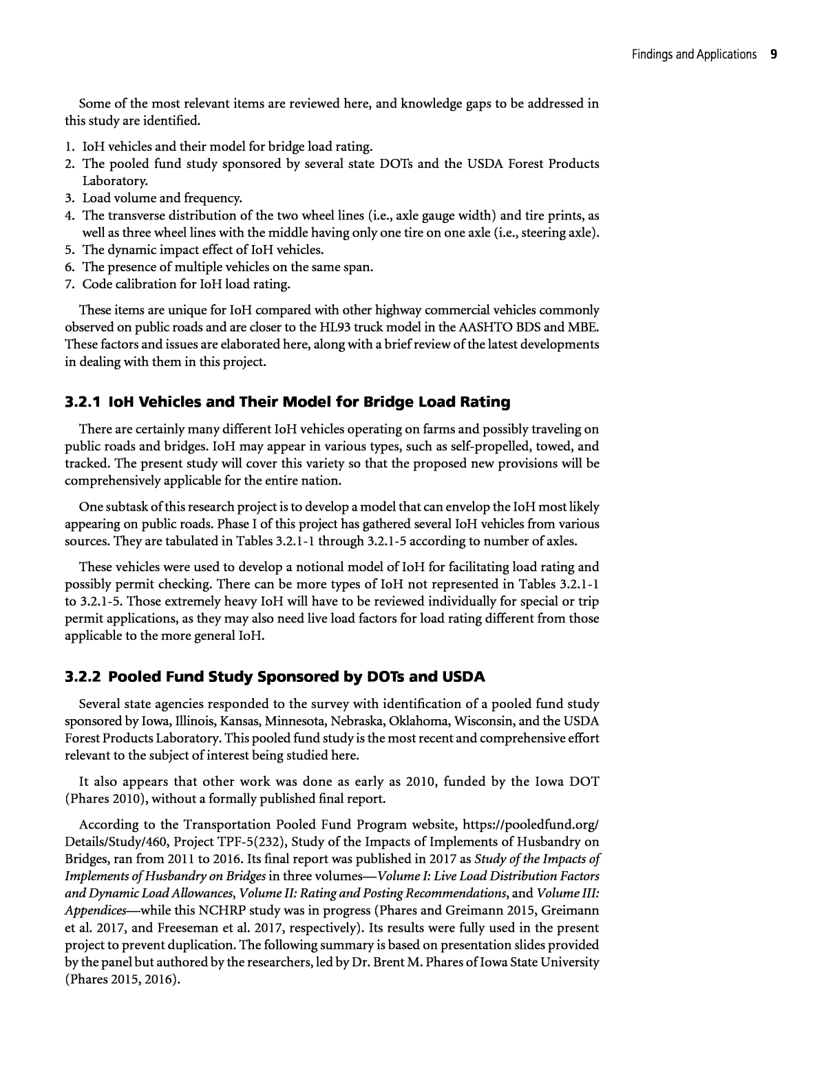
Findings and Applications 9 Some of the most relevant items are reviewed here, and knowledge gaps to be addressed in this study are identified. 1. IoH vehicles and their model for bridge load rating. 2. The pooled fund study sponsored by several state DOTs and the USDA Forest Products Laboratory. 3. Load volume and frequency. 4. The transverse distribution of the two wheel lines (i.e., axle gauge width) and tire prints, as well as three wheel lines with the middle having only one tire on one axle (i.e., steering axle). 5. The dynamic impact effect of IoH vehicles. 6. The presence of multiple vehicles on the same span. 7. Code calibration for IoH load rating. These items are unique for IoH compared with other highway commercial vehicles commonly observed on public roads and are closer to the HL93 truck model in the AASHTO BDS and MBE. These factors and issues are elaborated here, along with a brief review of the latest developments in dealing with them in this project. 3.2.1 IoH Vehicles and Their Model for Bridge Load Rating There are certainly many different IoH vehicles operating on farms and possibly traveling on public roads and bridges. IoH may appear in various types, such as self-propelled, towed, and tracked. The present study will cover this variety so that the proposed new provisions will be comprehensively applicable for the entire nation. One subtask of this research project is to develop a model that can envelop the IoH most likely appearing on public roads. Phase I of this project has gathered several IoH vehicles from various sources. They are tabulated in Tables 3.2.1-1 through 3.2.1-5 according to number of axles. These vehicles were used to develop a notional model of IoH for facilitating load rating and possibly permit checking. There can be more types of IoH not represented in Tables 3.2.1-1 to 3.2.1-5. Those extremely heavy IoH will have to be reviewed individually for special or trip permit applications, as they may also need live load factors for load rating different from those applicable to the more general IoH. 3.2.2 Pooled Fund Study Sponsored by DOTs and USDA Several state agencies responded to the survey with identification of a pooled fund study sponsored by Iowa, Illinois, Kansas, Minnesota, Nebraska, Oklahoma, Wisconsin, and the USDA Forest Products Laboratory. This pooled fund study is the most recent and comprehensive effort relevant to the subject of interest being studied here. It also appears that other work was done as early as 2010, funded by the Iowa DOT (Phares 2010), without a formally published final report. According to the Transportation Pooled Fund Program website, https://pooledfund.org/ Details/Study/460, Project TPF-5(232), Study of the Impacts of Implements of Husbandry on Bridges, ran from 2011 to 2016. Its final report was published in 2017 as Study of the Impacts of Implements of Husbandry on Bridges in three volumes—Volume I: Live Load Distribution Factors and Dynamic Load Allowances, Volume II: Rating and Posting Recommendations, and Volume III: Appendices—while this NCHRP study was in progress (Phares and Greimann 2015, Greimann et al. 2017, and Freeseman et al. 2017, respectively). Its results were fully used in the present project to prevent duplication. The following summary is based on presentation slides provided by the panel but authored by the researchers, led by Dr. Brent M. Phares of Iowa State University (Phares 2015, 2016).

Table 3.2.1-1. Two-axle IoH vehicles. No. Name/Type Remarks Total Weight (kips) 1 TerraGator 8400 Agricultural Truck 20 2 TerraGator 7300 Agricultural Truck 20 3 T1—John Deere 8430 30 4 T2—M. Ferguson 8470 22 5 T6—John Deere 8230 31 6 T7—Case IH 257 33 7 G1—Case IH 9330 27 8 T8—Case IH Steiger 485 53 9 John Deere Forage Harvester 37 10 S3—AGCO TerraGator 8204 32 11 R4—AGCO TerraGator 9203 38 12 R5—AGCO TerraGator 8144 32 13 R6—AGCO TerraGator 3104 42 14 MMI Feedtruck 33 15 Roto-Mix 31 16 Roto-Mix 49 17 Agricultural Floater Spreader 48 No. Name/Type Remarks Total Weight (kips) 1 John Deere 8520 & Kinze 1050 ROW Grain Cart 96 2 New Holland TD5050 & Kinze 1050 ROW Grain Cart 90 3 New Holland TD4040 & Kinze 1050 ROW 87 4 John Deere 8520 with Brent 1082 Grain Wagon 39 5 New Holland TD5050 with Grain Wagon Agricultural Truck 32 6 New Holland T4040 with Grain Wagon 29 7 John Deere 8520 & Kinze 1050 SOF Grain Cart 95 8 New Holland TD5050 & Kinze 1050 SOF Grain Cart 88 9 New Holland T4040 & Kinze 1050 SOF 86 10 TerraGator 2505 Agricultural Truck 43 11 Versatile 280 & Kinze 1050 ROW Grain Cart 101 12 Versatile 280 & Kinze 1050 SOF Grain Cart 100 13 Case 340B 64 14 John Deere 9200 & Kinze 1050 ROW Grain Cart 111 15 John Deere & Kinze 1050 SOF Grain Cart 110 16 John Deere 9200 with Brent 1082 Grain Wagon Agricultural Truck 53 17 Case 380 & Kinze 1050 ROW Grain Cart 110 18 Case 380 & Kinze 1050 SOF Grain Cart 108 19 Case 380 with Brent 1082 Grain Wagon 56 20 John Deere 9620 & Kinze 1050 ROW Grain Cart 114 21 John Deere 9620 & Kinze 1050 SOF Grain Cart 112 22 John Deere 9620 with Brent 1082 Grain Wagon Agricultural Truck 56 23 Case 600 with Grain Wagon 62 24 Case 600 & Kinze 1050 ROW 119 25 Case 600 & Kinze 1050 SOF 118 26 Versatile 535 with Grain Wagon 61 27 Versatile 535 & Kinze 1050 Row 118 28 Versatile 535 & Kinze 1050 SOF 117 29 John Deere 9620 & J&M 1075-22 Grain Cart 109 30 John Deere 8520 & J&M 1075-22 Grain Cart 92 31 John Deere 9200 & J&M 1075-22 Grain Cart 106 32 Versatile 280 & J&M 1075-22 Grain Cart 96 33 Case 380 & J&M 1075-22 Grain Cart 105 34 New Holland TD 5050 & J&M 1075-22 Grain Cart 85 35 New Holland T4040 & J&M 1075-22 82 36 Case 600 & J&M 1075-22 115 37 Versatile 535 & J&M 1075-22 114 38 Cotton Module Mover 68 39 S4—Homemade 28 40 S5—Homemade 28 41 G1—Case IH 9330 w/Parker 938 Cart 38 42 Tractor and Wagon 61 Table 3.2.1-2. Three-axle IoH vehicles.

Findings and Applications 11 Total Weight (kips) 1 Grain Semi Semitrailer 68 2 John Deere 8520 & Houle 2-Axle Tank Manure Tanker 85 3 New Holland TD5050 & Houle 2-Axle Tank Manure Tanker 79 4 New Holland T4040 & Houle 2-Axle Tank 76 5 John Deere 8520 & Balzer 6350 Narrow Manure Tanker 95 6 New Holland TD5050 & Balzer 6350 Narrow Manure Tanker 89 7 New Holland T4040 & Balzer 6350 Narrow 86 8 John Deere 8520 & Better-Bilt 3400 Manure Tanker 60 9 New Holland TD5050 & Better-Bilt 3400 Manure Tanker 53 10 New Holland T4040 & Better-Bilt 3400 50 11 John Deere 8520 & Better-Bilt 4950 Manure Tanker 78 12 New Holland TD5050 & Better-Bilt 4950 Manure Tanker 71 13 New Holland T4040 & Better-Bilt 4950 68 14 Versatile 280 & Better-Bilt 4950 Manure Tanker 82 15 Versatile 280 & Better-Bilt 3400 Manure Tanker 65 16 Versatile 280 & Balzer 6350 Narrow Manure Tanker 100 17 Versatile 280 & Houle 2-Axle Tank Manure Tanker 90 18 John Deere 9200 & Better-Bilt 4950 Manure Tanker 92 19 John Deere 9200 & Better-Bilt 3400 Manure Tanker 74 20 John Deere 9200 & Balzer 6350 Narrow Manure Tanker 110 21 John Deere 9200 & Houle 2-Axle Tank Manure Tanker 100 22 Case 380 & Better-Bilt 4950 Manure Tanker 91 23 Case 380 & Better-Bilt 3400 Manure Tanker 73 24 Case 380 & Balzer 6350 Narrow Manure Tanker 109 25 Case 380 & Houle 2-Axle Tank Manure Tanker 99 26 John Deere 9620 & Better-Bilt 4950 Manure Tanker 95 27 John Deere 9620 & Better-Bilt 3400 Manure Tanker 77 28 John Deere 9620 & Balzer 6350 Narrow Manure Tanker 113 29 John Deere 9620 & Houle 2-Axle Tank Manure Tanker 103 30 John Deere 9620 & Balzer 1250 Grain Cart 127 31 John Deere 8520 & Balzer 1250 Grain Cart 110 32 John Deere 9200 & Balzer 1250 Grain Cart 125 33 Versatile 280 & Balzer 1250 Grain Cart 115 34 Case 380 & Balzer 1250 Grain Cart 123 No. Name/Type Remarks 35 New Holland TD5050 & Balzer 1250 Grain Cart 103 36 New Holland T4040 & Balzer 1250 100 37 Case 600 & Better-Bilt 4950 101 38 Case 600 & Better-Bilt 3400 83 39 Case 600 & Balzer 6350 Narrow 118 40 Case 600 & Houle 2-Axle Tank 109 Table 3.2.1-3. Four-axle IoH vehicles. (continued on next page)

12 Proposed AASHTO Load Rating Provisions for Implements of Husbandry 41 Case 600 & Balzer 1250 133 42 Versatile 535 & Better-Bilt 4950 100 43 Versatile 535 & Better-Bilt 3400 82 44 Versatile 535 & Balzer 6350 Narrow 117 45 Versatile 535 & Houle 2-Axle Tank 108 46 Versatile 535 & Balzer 1250 132 47 Cotton Module Mover 88 48 T1—John Deere 8430 w/Houle Tank 45 49 T2—M. Ferguson 8470 w/Husky Tank 31 50 T6—John Deere 8230 w/ Husky Tank 46 Total Weight (kips) No. Name/Type Remarks Table 3.2.1-3. (Continued). No. Name/Type Remarks Total Weight (kips) 1 John Deere 8520 & Houle 3-Axle Tank Manure Tanker 103 2 New Holland TD5050 & Houle 3-Axle Tank Manure Tanker 96 3 New Holland T4040 & Houle 3-Axle Tank 93 4 Versatile 280 & Houle 2-Axle Tank Manure Tanker 108 5 Versatile 280 with Half-Full Houle 7300 Tank Agricultural Truck 77 6 John Deere 8520 & Better-Bilt 6600 Manure Tanker 98 7 Versatile 280 & Better-Bilt 6600 Manure Tanker 98 8 New Holland TD5050 & Better-Bilt 6600 Manure Tanker 91 9 New Holland T4040 & Better-Bilt 6600 88 10 John Deere 9200 & Better-Bilt 6600 Manure Tanker 112 11 John Deere 9200 & Houle 3-Axle Tank Manure Tanker 117 12 Case 380 & Better-Bilt 6600 Manure Tanker 111 13 Case 380 & Houle 3-Axle Tank Manure Tanker 116 14 John Deere 9620 & Better-Bilt 6600 Manure Tanker 115 15 John Deere 9620 & Houle 3-Axle Tank Manure Tanker 120 16 John Deere 9620 & Balzer 1500 Grain Cart 144 17 John Deere 8520 & Balzer 1500 Grain Cart 126 18 John Deere 9200 & Balzer 1500 Grain Cart 141 19 Versatile 280 & Balzer 1500 Grain Cart 131 20 Case 380 & Balzer 1250 Grain Cart 140 21 New Holland TD5050 & Balzer 1500 Grain Cart 119 22 New Holland T4040 & Balzer 1500 117 23 Case 600 & Better-Bilt 6600 120 24 Case 600 & Houle 3-Axle Tank 126 25 Case 600 & Balzer 1500 149 26 Versatile 535 & Better-Bilt 6600 119 27 Versatile 535 & Houle 3-Axle Tank 125 28 Versatile 535 & Balzer 1500 148 29 Cotton Module Mover (3-AxleTractor + CMC Trailer) 116 30 T7-Case IH 275 w/Houle Tank 59 Table 3.2.1-4. Five-axle IoH vehicles.

Findings and Applications 13 No. Name Remarks Total Weight (kips) 1 John Deere 8520 with 2 Empty Nuhn QT Quad Tanks Agricultural Truck 52 2 John Deere 9200 with 2 Empty Nuhn QT Quad Tanks Agricultural Truck 66 3 New Holland TD5050 with 2 Empty Nuhn QT Quad Tanks 45 4 New Holland T4040 with 2 Empty Nuhn QT Quad Tanks 42 5 Case 380 with 2 Empty Nuhn QT Quad Tanks Agricultural Truck 69 6 John Deere 9620 with 2 Empty Nuhn QT Quad Tanks Agricultural Truck 73 7 Case 600 with 2 Empty Nuhn QT Quad Tanks 79 8 Versatile 535 with 2 Empty Nuhn QT Quad Tanks 78 9 T8—Case IH 485 w/ Houle Tank 78 Table 3.2.1-5. Six-axle IoH vehicles. The pooled fund study included load tests of 19 bridges using four IoH vehicles and one semitrailer (3S2 type) as a typical highway vehicle to load the bridges. The study also used the finite element method (FEM) for analysis of these bridges, along with another 174 bridges and 121 IoH vehicles. The following major recommendations are included in Volume I (Phares and Greimann 2015): 1. In general, AASHTO BDS were conservative for live load distribution factors in designing and rating slab-on-girder bridges for husbandry vehicles. 2. The empirical equations provided a good estimation of the live load distribution factors and are recommended for consideration in designing and rating slab-on-girder bridges for husbandry vehicles. However, the equations do have limitations, primarily because few bridges were analyzed for some bridge types. 3. This study can be extended to other bridge types built on secondary roadways and subjected to husbandry vehicle loadings. Additionally, more steel–concrete, steel–timber, and timber–timber bridges should be added to increase confidence in the empirical equations. 4. Because limited dynamic data were available, further investigation of the IM of husbandry vehicles would be appropriate. Volume II of the pooled fund study also included Section 7, “Summary and Conclusions for Rating and Posting Recommendations” (Greimann et al. 2017). However, its contents are more narrative statements about how the study was conducted than recommendations. Its structure is far different from the four major recommendations from Volume I. The only exception is this paragraph: Following AASHTO MBE (Manual for Bridge Evaluation) and MUTCD (Manual on Uniform Traffic Control Devices), possible bridge restriction signs, including speed limit sign and load posting sign, are proposed. Using a separate restriction sign for farm vehicles is considered to be a practical way to ensure the bridge safety when subjected to implement of husbandry loads while avoiding over posting for other types of vehicles. Note also that Volume III (Freeseman et al. 2017) includes only appendices for many details. It does not include any recommendations. This pooled fund study was important to the present NCHRP study, especially the unpublished data that represent an unprecedentedly large bridge load test data set. This data set was also most directly relevant to this NCHRP study compared with all other load test data sets available because the data were obtained using IoH vehicles on local and short-span bridges of particular interest in the United States.

14 Proposed AASHTO Load Rating Provisions for Implements of Husbandry 3.2.3 Load Volume and Frequency Load volume and frequency of IoH could greatly affect the live load model and load factor for bridge load rating. The current AASHTO MBE’s live load factors were derived using truck- load data (Nowak 1999; Moses 2001) from weigh stations in Canada by weighing stationary trucks. The data do not have recorded cases of multiple vehicles in motion present on the same span. Such load configurations represent governing loading and thus are critical for strength- limit states in bridge load rating. This is one reason the AASHTO MBE allows refinement of live load factors for local condi- tions based on WIM data. Apparently, the presence of multiple vehicle loads is a function of load volume and frequency—more vehicles crossing the bridge within a given period will more likely cause the presence of multiple vehicles on the same span. About 10 states have pursued refinement so far, as summarized in Fu, Chi, and Wang (2019). Some background work in this regard for NCHRP Project 12-110 was published in Fu (2013); Fu and You (2009, 2011); Fu and van de Lindt (2006); and Fu, Chi, and Wang (2019). To understand real IoH on roads, an effort was made in this project to maximize use of WIM data or other weight data of IoH on roads. An example of recorded IoH on roads is shown in Figure 3.2.3-1. To this end, the Wisconsin DOT also has provided IoH permit application data. 3.2.4 Transverse Distribution of the Two and Three Wheel Lines IoH have different dimensional characteristics, particularly from typical highway vehicles notionally modeled by the HL93 truck. This is especially true with respect to the transverse distance between the two wheel lines (6 ft in the HL93 truck in the current AASHTO BDS and MBE). Some IoH vehicles have three wheel lines, because their steering axle has only one tire in the middle between the other two wheel lines. The transverse distance between wheel lines is sometimes referred to as the “axle gauge width” or “gauge width” (GW) in the literature. It affects load distribution among the parallel longi- tudinal bridge members (such as girders or stringers) supporting a bridge deck, which is determined or estimated using the load distribution factor in the current AASHTO BDS for both design and load rating. The pooled fund study has made progress with respect to the Figure 3.2.3-1. An example IoH recorded in motion in Minnesota with WIM technology (Source: Minnesota DOT).

Findings and Applications 15 distribution factors for IoH in or around the Iowa area by analyzing 121 IoH vehicles and by physically testing five local bridges for finite element model calibration as well as for the dynamic impact of IoH (Seo, Phares, and Wipf 2014; Phares 2015, 2016; Seo and Hu 2015; Abu-Hawash and Phares 2016). Empirical formulas for live load distribution factors were developed from the study to account for the effect of axle gauge width (Phares and Greimann 2015). As stated in Recommendation 3 (Phares and Greimann 2015): 3. This study can be extended to other bridge types built on secondary roadways and subjected to husbandry vehicle loadings. Additionally, more steel–concrete, steel–timber, and timber–timber bridges should be added to increase confidence in the empirical equations. The scope of span type here apparently needs to be expanded for wider coverage for the entire nation. There is no doubt that the three types the pooled fund study focused on are among those of concern with respect to IoH vehicles. The survey results summarized in Section 3.1.1 have indicated so, also including other types, such as reinforced concrete and timber slab spans, reinforced concrete T-beam spans, and prestressed concrete beam spans. Other parameters of IoH vehicles could affect live load distribution among parallel bridge members, such as longitudinal girders and beams. Such parameters may be tracked wheels, variable gauge widths, single tires (i.e., single wheels) in one axle, multiple tires in one wheel (e.g., four tires on one axle), and so on. WIM data do provide axle (and sometimes wheel) weights, but not tire size nor whether wheels are tracked. There have not been previous studies on the effects of such IoH parameters on live load distribution in bridge members. Tools are thus needed for engineers to deal with these parameters in IoH load rating. 3.2.5 Dynamic Impact Effect of IoH Vehicles The dynamic impact effect of IoH may be different from other typical highway vehicles, because of their distinct configurations in both longitudinal and transverse directions. In addition, other factors and their combinations, such as vehicle speed, roadway surface condition, vehicle suspension system characteristics, natural frequencies in a complex dynamic system, and damping properties of the coupled bridge-vehicle system (which also varies during bridge crossing), could contribute to this difference. Because so many parameters are involved in dynamic behavior and effects to bridge members, the most reliable approach to assessing the dynamic impact effect of IoH is in situ physical testing. Numerical modeling, such as finite element analysis alone, has to be based on many assumptions that are not readily verifiable. Without a budget for such physical testing, NCHRP Project 12-110 performed a literature search and review regarding the effect of moving trucks on dynamic load in roadway bridge members. Before the review is presented, it is worth noting that the dynamic load allowance, IM, and the impact factor, I, in the AASHTO BDS and Standard Specifications for Highway Bridges (SSHB) are often different from dynamic amplification obtained via physical testing. However, IM and I have been confused in the literature, particularly when they are directly compared. IM for LRFR and I for LFR are intended to be used in design and evaluation of the structure, with the intention to envelop the dynamic effect of the load along with the static load effect. Accordingly, IM for LRFR and I for LFR are supposed to be applied to the standard design or evaluation load model at the most severe position to generate a notional load effect believed to envelop maximum credible load effect for the intended period (life for design, or inspection interval for evaluation). Note that IM factor or I refer to maximum static load effects. Previous load tests have shown IM and I decreasing with static response increase. Namely, IM/I is lower for heavier loads.

16 Proposed AASHTO Load Rating Provisions for Implements of Husbandry On the other hand, the dynamic amplification factor or impact factor obtained from physical testing is a percentage (or a fraction) increase from the static response for the total response of the applied load. The referenced static response is usually not the factored load for design or evaluation. As a matter of fact, it is much lower than the factored design load effect. For example, the HL93 truck is actually beyond the current U.S. federal legal load limit, according to FBF. The test load, rather, is often a legal load so that the test vehicle may travel to the test site without a permit. It is thus much lower than the HL93 truck and, of course, even lower than the factored design load. In the practice of field load testing to a bridge span, the dynamic total response is recorded when the vehicular load is applied at a speed of interest, or at a limit determined by the vehicle or road surface condition. In another run, the static response is recorded with a stationary load or at a speed close to 0, a crawl speed (e.g., 5 mph), though crawl speeds are difficult, if not impossible, to control exactly. As such, the so-called static run at a crawl speed should be more precisely referred to as a “pseudo-static run.” In addition, one load path of a test is unable to induce the maximum possible load effect in one or all components of concern, whether a dynamic or a pseudo-static run. Multiple such runs may still be unable to accomplish the maximum possible load effect if these runs are not carefully designed. The dynamic load allowance IM in AASHTO BDS (i.e., the difference between the dynamic total response and the static response at zero speed) is meant to envelop the dynamic load allowance for all cases possible and all structural components of concern. For bridge design, “IM” refers to the standard design load model (the HL93). For evaluation, “IM” refers to the standard evaluation load model (such as the AASHTO legal loads). Therefore, it is important to fully comprehend available test results when recommending IM or I in SSHB when developing new provisions for LRFR and LFR. However, many publications in the literature do not differ- entiate the IM or the I from the measured dynamic amplification factor. When developing the IM factor and I for the proposed LRFR and LFR provisions for IoH, it is important to carefully determine what previous publications may have intended. Note also that the review here uses the following definitions, consistent with the AASHTO definitions for dynamic load allowance IM (BDS) and impact factor I (SSHB): IM IM factor Static Load Effect according to BDS (3.2.5-1)( )= × I Impact Factor according to SSHB (3.2.5-2)( )= As seen, the IM factor is conceptually equivalent to I, although the former is given as 0.33 and the latter is capped at 0.30 in BDS and SSHB for design. Szurgott et al. (2011) reported a study for the Florida DOT on dynamic amplification of permit trucks using physical testing. The test structure was a 1999-built prestressed concrete beam bridge, with three simple spans each 71.2 ft long. Three test vehicles were used to load the bridge for both dynamic and static responses of strains and deflections. The loading trucks’ configurations are shown in Figure 3.2.5-1. The bridge approach depression, combined with a distinct joint gap between the asphalt pavement and the concrete deck (Figure 3.2.5-2), triggered significant dynamic responses of the bridge-vehicle system. Similar dynamic vibrations were observed and recorded when the permit vehicles were driven over speed bumps. Time histories of relative displacements, accelerations, and strains were recorded for selected locations of the bridge-vehicle system. The analysis of experimental data allowed for assessment of actual dynamic interactions

Findings and Applications 17 between the vehicles and the speed bumps, as well as dynamic load allowance factors for the bridge. Szurgott et al. (2011) gave the following conclusions: 1. Surface imperfections of bridge decks, bridge approach depressions, potholes, and joints between asphalt pavements and concrete bridge decks were found to trigger a dynamic response of the vehicle–bridge system. A good maintenance plan, aimed at controlling and reducing these imperfections, may significantly reduce dynamic loading of bridges, improving their “health” and service lives. 2. Given the surface imperfections, several factors were identified that can either mitigate or magnify the dynamic response of the vehicle–bridge system and resulting dynamic load allowance factors: a. Modern vehicle suspensions, with efficient spring and damping characteristics, are effective in controlling vibrations and the resulting dynamic load allowance factors. b. Multiple axles with double wheels and a longer wheelbase help to more evenly distribute the load and to control vibrations. Figure 3.2.5-1. Configurations of heavy load vehicles: (a) truck tractor, 117 kips; (b) Terex T-340 crane, 61 kips; and (c) Florida DOT truck, 71 kips (Szurgott et al. 2011). Figure 3.2.5-2. Noted elevation difference between bridge deck and pavement (Szurgott et al. 2011).

18 Proposed AASHTO Load Rating Provisions for Implements of Husbandry c. Vehicle mass and speed are directly proportional to dynamic effects of the vehicle–bridge system that they trigger. However, they are not necessarily as important as other factors, such as suspension and wheelbase. d. Poor, loose, and slack cargo tie-downs were found to trigger a hammering load effect, significantly magnifying the dynamic response of the vehicle–bridge system. Deng et al. (2014) conducted a review on dynamic impact factor for highway bridges. The study focused on design and evaluation specifications in several countries. The AASHTO codes specify a maximum IM factor of 0.33 for design and various values up to 0.30 for evaluation, depending on road surface condition. Note also that the AASHTO SSHB has the design impact factor I as a function of span length and capped at 0.30. Other countries specify the IM factor in various ways: • The Ontario bridge design code has IM factor as a function of the first flexural frequency but capped at 0.40. • The current Chinese bridge and culvert design code still specifies the IM factor value as a function of span length; the code used to have the IM factor as a function of the fundamental frequency as well. • The New Zealand bridge design code also gives the IM factor as a function of span length, with a maximum of 0.30. • The Australia bridge design code prescribes a table of IM factors depending on the load (e.g., wheel load, axle load, heavy platform load) being designed for. The heavier the load is, the lower the IM factor value is, running from 0.1 to 0.4. • The Eurocode prescribes the IM as a function of not only span length but also number of lanes, as well as load effect—moment or shear. The fewer the lanes, the larger the IM factor, and the shorter the span, the larger the IM factor. The maximum value is 0.70 for moment, single lane, and span length shorter than 16 ft, which appears to be a special situation among many other cases (two lanes, longer spans, and so on). • The British bridge design code specifies a constant 0.25 value of IM factor for all cases. • The Japanese bridge design code also specifies the IM factor as a function of span length and the bridge component’s material (steel, reinforced concrete, or prestressed concrete), as well as truck load or lane load. It appears that the IM factor (or impact I) is largely in the range of 0.1 to 0.3 among these design codes. Note also that most of these countries do not have a formal bridge evaluation code. As such, any evaluation will have to use the design IM factor to be consistent and appropriate. Han et al. (2015) performed load testing on a prestressed concrete T-beam bridge of six continuous spans, each 82 ft (25 m) long. The load was applied using trucks weighing about 64.4 kips (29.2 metric tons) at speeds between 18.6 and 21.8 mph. One-lane and two-lane loadings were used. The ratio of dynamic response to static response (i.e., dynamic amplifica- tion) was found to be at a value of IM factor below 0.33 in the AASHTO BDS, except for very poor pavement condition. Typical response records are shown in Figure 3.2.5-3. Harris, Civitillo, and Gheitasi (2016) presented a recent research effort on highway bridge members’ in situ dynamic impact effect. The bridge system tested in Virginia was a 44 ft span with eight hybrid composite beams in the cross section. Hybrid composite beams are made of a fiber-reinforced polymer (FRP) I-beam section hybrid with reinforced concrete, as shown in Figure 3.2.5-4. A range of dynamic amplification factor was found between 6% and 75%. The high percentages are associated with less-severely loaded beams close to the fascia. Holden, Pantelides, and Reaveley (2015) presented another recent study of dynamic test- ing for an 88.2 ft long bridge in Utah with 12 prestressed AASHTO Type IV girders in its cross section. This study was to understand the bridge’s dynamic amplification in response to five different truck-load configurations. The impact factor for IM was found between 9% and 19%,

Findings and Applications 19 Figure 3.2.5-3. Recorded dynamic responses of deflection with (a) one-lane loading and (b) two-lane loading (Han et al. 2015). Figure 3.2.5-4. Dynamically tested hybrid composite beams (Harris, Civitillo, and Gheitasi 2016). depending on truck weight and thus the static response. The study concluded that higher truck weights lead to lower IM factor values. IM factor was also found to increase with the truck speed used to load the span. For IoH vehicles’ dynamic load allowance IM or its factor in percentage, the pooled fund study is relevant to the present NCHRP study, particularly Volume I that focuses on dynamic load allowance (Phares and Greimann 2015) and Volume III that reports many details of the load tests (Freeseman et al. 2017). These tests used two sets of different IoH vehicles in 2010 and 2011 to dynamically load 19 local bridges. Each of the two sets included four IoH vehicles: (1) a TerraGator with one or two dual-tire axles plus a single-tire steering axle, (2) a tractor grain wagon with a two-axle tractor hauling a one-axle grain cart, (3) a tractor honey wagon consisting of a two-axle tractor hauling a three-axle half-full tank, and (4) another tractor honey wagon of a two-axle tractor hauling two empty tanks, each on two axles. The vehicles are shown in Figure 3.2.5-5. Between the two vehicle sets, these four vehicles had differences in gross vehicle weight and length (Freeseman et al. 2017). The load tests also included a typical semitrailer for comparison with the IoH vehicles, which is displayed in Figure 3.2.5-6. The dynamic tests used a nominal speed of 10 to 25 mph, and the pseudo-static test a nominal 3 mph speed (Freeseman et al. 2017). The dynamic speed was chosen considering the speed limit of the site. Figures 3.2.5-7 through 3.2.5-9 show the typical pavement material and condi- tion of the tested bridges.

20 Proposed AASHTO Load Rating Provisions for Implements of Husbandry TerraGator Honey Wagon Tractor Grain Wagon Honey Wagon with two tanks Figure 3.2.5-5. IoH loading vehicles used in pooled fund study (Freeseman et al. 2017). Semi Truck Figure 3.2.5-6. Loading semitrailer used in pooled fund study (Freeseman et al. 2017).

Findings and Applications 21 Figure 3.2.5-7. Typical road surface of load-tested bridge (Iowa Bridge 68790, with timber beams supporting timber deck): overall view (top) and closer view (bottom) of timber deck surface deterioration (pooled fund study, unpublished data set). Figure 3.2.5-8. Typical road surface of load-tested bridge (Iowa Bridge 126231, with steel beams supporting timber deck) (pooled fund study, unpublished data set).

22 Proposed AASHTO Load Rating Provisions for Implements of Husbandry Figure 3.2.5-9. Typical road surface of load-tested bridge (Iowa Bridge 126252, with steel beams supporting timber deck): overall view (top) and closer view of approach surface deterioration (bottom) (pooled fund study, unpublished data set). A total of 19 local bridges were used in these load tests. They are 5 steel beams/concrete deck bridges, 11 steel beams/timber deck bridges, and 3 timber beams/timber deck bridges. Ten can carry only one lane of traffic, two can carry two lanes, and seven have a width narrower than 24 ft but can accommodate two lanes of traffic at a low speed. The traditional load test approach was used to extract the IM factor as follows. IM Factor Maximum total response Maximum pseudo-static Response 1 (3.2.5-3)= −

Findings and Applications 23 Note that the total response in Equation 3.2.5-3 was referred to as “dynamic strain” and the pseudo-static response was referred to as “static strain” in Phares and Greimann (2015) and Freeseman et al. (2017). However, the dynamic strain and pseudo-static strain were recorded when the vehicle crossed the bridge at two different speeds, the dynamic one supposedly being faster than the pseudo-static one. Since the strains were done in two separate runs and at two different speeds, matching the two at respective maximum response for applying Equation 3.2.5-3 can be challenging, if not impossible. First, the nominal speeds of the two runs cannot be kept respectively constant. In other words, the intended constant or nominal speed for a run actually became variable speeds in the field test, as seen in the digital data, likely because the speed was manually controlled by the driver, not by a computer. In addition, the intended identical path for both runs was almost impossible to realize, so that expected maxima might not be observed at all. For example, the maximum in the dynamic strain curve might be observed at the second axle loading the sensored beam, while in the pseudo-static the maximum occurred at a third axle or vice versa. This situation made Equation 3.2.5-3 impossible to apply because it is intended to use the maxima from the same axle load loading the same sensored member. Figure 3.2.5-10 is a comparison of recorded pseudo-static and dynamic strains, taken from Freeseman et al. (2017) for Steel–Concrete Bridge 1, identified as Bridge 77560 in Iowa. The strains were recorded using the strain gauge on Girder 5’s bottom flange when loaded with the tractor grain wagon. Girder 5 was at the cross section’s centerline of this 11-girder bridge. As seen in Figure 3.2.5-10, the first and second peaks at around 7 and 12 ft matched well between the dynamic and pseudo-static strains, but the third peak around 21 and 24 ft is off. Note that the raw data have equal time intervals at a frequency of 100 data points per second, 0 0 10 20 30 40 50 60 70 80 5 10 15 20 Truck Position (ft) St ra in - G ir de r 5 (l d) 25 30 35 40 Tractor with Grain Wagon (Static) Tractor with Grain Wagon (Dynamic) Figure 3.2.5-10. Comparison between pseudo-static and dynamic strains for Iowa Bridge 77560 (Freeseman et al. 2017).

24 Proposed AASHTO Load Rating Provisions for Implements of Husbandry or one point per 0.01 second. Data points had to be converted to distance as shown in Figure 3.2.5-10, using the respective speeds of the two runs. Both speeds were intended to be constant, but realistically they were not. It is also seen in Figure 3.2.5-10 that the maximum dynamic strain at about 12 ft is a little lower than the maximum pseudo-static strain, similar to the other two peak dynamic strains at about 7 ft and 24 ft. As a result, the IM factor formulated in Equation 3.2.5-3 will turn out to be negative. It would mean that the dynamic load allowance IM should be negative, which makes no practical sense for bridge design or evaluation. Also note that the three peaks in Figure 3.2.5-10 correspond to the three axles of the loading tractor grain wagon, one of the four IoH shown in Figure 3.2.5-5. The pseudo-static strain actually exhibits more dynamic or cyclic motion than the dynamic strain in Figure 3.2.5-10, especially near the third axle (i.e., the grain cart axle). This oscillation is better displayed and more visible in Figure 3.2.5-11, which uses all data points available in the unpublished pooled fund study data set and denotes the bottom flange of Girder 5. This oscillation illustrates that pseudo-static response is actually not static. Shown in Figure 3.2.5-11 is the contrast between the pseudo-static strain of another strain gauge attached to the same beam’s top flange in the longitudinal direction, parallel to the bottom flange’s strain gauge. Both strains were recorded simultaneously when the loading tractor grain wagon crossed the bridge. The strain-response magnitude in the top flange is much lower while still exhibiting noticeable oscillation or dynamic behavior, especially near the third axle. These two pseudo-static strain records are indeed dynamic by nature. As such, they could also be analyzed to extract the IM factor for the vehicle speed. When such an analysis is performed, the two records, however, will consistently give different IM factor values using the same equation, Equation 3.2.5-3. This can be clearly seen by the relative weight of the dynamic response within the total response, as noted in Figure 3.2.5-11. For the bottom flange strain record, the IM factor or I is about 10% according to Equation 3.2.5-3 Data Point M ic ro st ra in - G ird er 5 Bottom Flange Top Flange Figure 3.2.5-11. Comparison of dynamic response portion in high and low static responses for Iowa Bridge 77560 (pooled fund study, unpublished data set).

Findings and Applications 25 at the third peak (corresponding to the grain cart axle load). For the top flange strain record at a much lower level compared with the bottom flange, the IM factor or I is about 33% at the third peak for the same axle load. Apparently, 10% should be used as a candidate for IM factor or I to be included in the specifications, along with other such candidates from other tests. The 33% value should accordingly be excluded for further consideration, because it is associated with a much lower static response, not consistent with the definition for IM and I in AASHTO BDS and SSHB, respectively. This analysis highlights that lower total response (or pseudo-static response) leads to higher IM factor and I. This has been observed in previously reported load tests, as discussed. It also dictates that IM factor extraction should focus on the maximum static response or maximum total response, for which IM or I is intended to be applied in design and evaluation specifications. Using lower responses for such extraction could lead to overestimated IM factors or I values, inconsistent with their definitions in the specifications. Overestimating these values from test- ing does offer some information on dynamic amplification, but they are not of interest when specification development is focused. Such demonstrated issues with the traditional IM factor extraction approach used in the pooled fund study were present in many previously reported studies. The issues might also exist in the studies reviewed earlier in this section. Nevertheless, it is difficult to illustrate them because most papers and reports do not offer test data details, as done in Freeseman et al. (2017). This NCHRP study will address these issues using a different approach. 3.2.6 Presence of Multiple Vehicles on the Same Span The presence of multiple vehicles on the same span is important because such a confi- guration represents the load case critical to bridge safety. Multiple presence may be lateral or longitudinal. Lateral multilane occupation by vehicles is modeled by the multiple presence factor in the current AASHTO BDS for design and is referred to in the AASHTO MBE for load rating. Theoretically, the live load factors in the AASHTO BDS and MBE are supposed to cover the possible longitudinal presence of multiple vehicles. Nevertheless, the presence of multiple vehicles had only been covered implicitly until recent studies using WIM data (Fu and You 2009, 2011; Fu, Liu, and Bowman 2013). Currently, only WIM data can provide reliable information on how often these critical load cases may occur, which need to be focused on in bridge load rating and design for strength- limit states. However, in most past studies for calibrations of the AASHTO BDS and MBE, this was impossible because stationary truck-weight data from Canadian weigh stations were used, rather than WIM data. More critically, WIM data need to be used with well-designed and -tested computer software processing programs to extract real and critical cases of multiple vehicles and arrive at needed statistics for code calibration. The research team has successfully accomplished these steps with verification (Fu and You 2009, 2011; Fu, Liu, and Bowman 2013), and the resulting tools have been successfully used in research projects for Michigan DOT (Fu 2010, 2013) and Illinois DOT (Fu, Chi, and Wang 2019). These tools were also used in the present project to reliably find the maximum load combination statistics for calibration of the load factors for IoH. For certain low-traffic roads and one-lane roads common in local systems, a multiple presence factor may not be needed because such a scenario does not take place. When truck traffic is low (e.g., average daily truck traffic [ADTT] < 100), WIM data have shown that the presence of multiple trucks on the same bridge span never occurs. In addition, if only one lane is available, the transverse presence of multiple trucks becomes impossible or not applicable.

26 Proposed AASHTO Load Rating Provisions for Implements of Husbandry How to account for the presence of multiple vehicles on the same span has not received attention in previous studies on IoH (Seo, Phares, and Wipf 2014; Dahlberg 2015; Phares 2015; Phares and Greimann 2015; Seo and Hu 2015; Freeseman et al. 2017; Greimann et al. 2017). As mentioned earlier, new WIM data from Minnesota have recorded IoH vehicles with images (e.g., Figure 3.2.3-1). This valuable source of data was identified using the lead obtained in the response to our questionnaire. Maximized use of available WIM data is exercised in this project to understand the possible presence of multiple IoH vehicles or IoH vehicles along with other highway vehicles. Such understanding will allow realistic and reliable provi- sions and protocols for load rating IoH. 3.2.7 Code Calibration for IoH Load Rating One subtask in NCHRP Project 12-110 was to derive live load factors for IoH to be part of the new LRFR and LFR provisions and protocols. In the literature, this process is referred to as “code calibration to a target bridge safety.” Structural reliability-based code calibration itself has been advancing largely because more vehicle weight measurement data are becoming available. Analyses of these data have also challenged assumptions used in past calibrations. The original calibrations for AASHTO MBE and BDS used limited stationary truck-weight data from Canada. A review of the state of the art and the practice for load-rating calibration is offered next, along with possible methods to advance in this project. A complete review can be found in Fu, Chi, and Wang (2019), including calibration efforts for bridge design provisions. New York State DOT Study, 1997 Fu and Hag-Elsafi (1997) in a New York State DOT project conducted the earliest research developing state-specific live load factors for overweight permit trucks, using truck-weight data and reliability-based calibration. Available New York permit truck-weight data were used to develop the live load factors for annual and trip permits. It was this effort that introduced the concept of lower live load factors for heavier trucks. This concept was referenced and adopted in NCHRP Research Report 454 (Moses 2001) and, in turn, in the AASHTO Guide Manual for Condition Evaluation and Load and Resistance Factor Rating (LRFR) of Highway Bridges in 2003. The study by Fu and Hag-Elsafi (1997) was also the first research effort that treated real permit loads separately to derive load factors for them. The report was cited in the LRFR- calibration report NCHRP Report 454 (Moses 2001), which did not use newer truck-weight data than that in LRFD calibration from Canada. This approach was also used later in NCHRP Project 20-07/Task 285 (Sivakumar and Ghosn 2011) for recalibration of the AASHTO MBE for permit load. The use of lower live load factors for heavier trucks has since been carried over to current LRFR through all three AASHTO MBE editions in 2008, 2011, and 2018. NCHRP Projects 12-46 and 20-07/Task 285 In NCHRP Project 12-46, Moses (2001) conducted calibration of live load factors for bridge load rating, as documented in NCHRP Report 454. Live load factors were recommended for permit load in the resulting AASHTO LRFR guide manual published in 2003. The recommen- dation was based on judgment and reference to earlier experiences in Fu and Hag-Elsafi (1997). Original calibration for legal loads in NCHRP Report 454 was based on the same Canadian truck-weight data used in the LRFD calibration, without recorded behavior of trucks in motion such as multiple vehicles on the span. Therefore, the same assumptions used in LRFD calibration had to be used in this project. They included, but were not limited to, the side-by-side probability of 1/15 that was later shown

Findings and Applications 27 to be overconservative by WIM data in NCHRP Project 12-63 (Sivakumar et al. 2007). A load model was used in NCHRP Report 454, including two independent random variables, each repre- senting one lane of truck weight. Several years later, NCHRP Project 20-07/Task 285 (Sivakumar and Ghosn 2011) was established to recalibrate the LRFR specifications for permit rating. The approaches to recalibration in NCHRP 20-07/285 (Sivakumar and Ghosn 2011) were advanced from those in NCHRP Report 454 (Moses 2001). NCHRP 20-07/285 used WIM data with the permit load separated, as in Fu and Hag-Elsafi (1997, 2000). The report also used a different future maximum value projection (to predict 5-year future maximum load) from projections used in NCHRP Report 454 and LRFD calibration. This approach’s main concepts are based on the protocols recommended by NCHRP Project 12-76 (Sivakumar, Ghosn, and Moses 2008; Sivakumar et al. 2011), although the NCHRP 12-76 protocols were meant for bridge design. These changes in calibration approaches also highlight the limitations of those used in the original LRFD and LRFR calibrations, as well as the advancement in technology associated largely with WIM data becoming available. NCHRP Report 454 noted the following reporting calibration for the AASHTO bridge evaluation specifications: Other parts of the Ontario data that should be kept in mind in considering the accuracy of load projections are as follows: • The data recorded is a 2-week sample. Any other 2-week sample would have a different outcome because of statistical variability and also seasonal influences on truck movements. • Heavy trucks avoid static weigh stations, and the degree to which this avoidance occurred in the recorded sampling is unknown. • Truck weights have changed over time. A repeat of the Ontario trial recently, some 20 years after the first weighings, showed increased truck weights in terms of the maximum bridge loadings (Moses 2001, 15). NCHRP Project 12-63 NCHRP Project 12-63 is another project relevant to understanding how IoH trucks may simultaneously appear on the same bridge span, referred to here as “cluster appearing.” However, in the literature, the phrase “side by side” has been used for this phenomenon but without explicit definition. “Side by side” appears to refer to the loading situation when two trucks in different lanes have their headway distance equal to zero. However, this situation has rarely been recorded in WIM data, if ever. The real situation of concern is when two or more trucks are in a cluster simultaneously on the same span and with small headway distance from one another. Such clustering is focused on here because cluster appearing represents the governing loading for strength-limit states in load-rating bridge spans. NCHRP Report 575 (Sivakumar et al. 2007), in which the results of NCHRP Project 12-63 were published, documented WIM data collected from highways by Fu, one of the coauthors. WIM data with 0.01-second time-stamp resolution were gathered and analyzed for the first time in history. Such data are critical in understanding the truck-load occurrences in cluster. Highways in Idaho, Michigan, and Ohio were specially instrumented to acquire such data. The so-called side-by-side loading with zero headway distance was never recorded, partially because the time-stamp resolution was 0.01 second and no two time stamps of heavy trucks were ever identical. In other words, no two trucks in different lanes ever arrived at the same cross section of a bridge span at the same time, up to the resolution of 0.01 second. The multiple presence data then were arranged by headway distance to quantitatively describe the real behavior. Table 15 in NCHRP Report 575 prepared by Fu is a typical example of the measurement result for one of the three sites in Michigan. The table shows that if headway less than 5 ft is

28 Proposed AASHTO Load Rating Provisions for Implements of Husbandry defined as a side-by-side occurrence, its probability is averaged at 0.045% for an ADTT of 4,214. This value is negligible compared with the 1/15 (6.7%) value used in original LRFD calibration for a maximum ADTT of 5,000. Further, if headway of less than 15 ft is accepted as a side-by-side occurrence, then an averaged 0.10% probability is observed. Moreover, if the acceptable headway is increased to 60 ft, as in the most generous case (also conservative because of an overestimated load effect), an averaged 2.11% probability was observed, still lower than 1/15, or 6.7%. This 60-ft headway should not be accepted as the side-by-side occurrence for all spans and all load effects. For example, when the first truck is in the midspan area of a simple span, inducing a maximum moment, a second truck with a 60-ft headway will be off the span if the span length is 90 ft or shorter. Thus, the second truck will contribute nothing to the total midspan moment; therefore, the so-called side-by-side configuration does not form. Instead, the “generous” 60-ft headway in NCHRP Report 575, Table 15, was used to show that the 1/15 side-by-side probability was an extremely conservative overestimate. It was not meant to be the definition for the side-by-side configuration. Nevertheless, this 60-ft headway since then has been misused as the definition of side-by-side loading in many reports in the literature. Note also that the Idaho and Ohio data obtained in NCHRP Project 12-63 have shown the same behavior as Table 15 in Sivakumar et al. (2007) shows for the Michigan site on US-23 near Detroit. Oklahoma DOT Study The Oklahoma DOT was implementing a statewide load-rating program for in-service bridges using the LRFR methodology. The objective of the project was to define state-specific live loads and/or load factors using recent truck-weight data collected from both Interstate and non-Interstate WIM sites in Oklahoma for use with the LRFR methodology (Sivakumar 2011). WIM data from nine sites were used in this study, with the longest history of 640 days and the shortest of 59 days. The overall average was 478 days. The approach of NCHRP Project 12-76 (Sivakumar et al. 2011) was used for calibration. The project report recommended that for Interstate highways, the three AASHTO legal trucks (Types 3, 3S2, and 3-3) be used for load rating. For state routes, five vehicles were recommended for load rating: Types 3S2 and 3-3, SU4, SU5, and SU6. With these recommendations, no change to the AASHTO live load factors was needed, as recommended in the report. Yet AASHTO live load factors for legal-load rating in MBE have been decreased since then. In addition, the relative calibration recommended by Moses (2001) was used in the study. This approach will be used in the present study, as in Section 3.7.2, Calibration Approach. New York State DOT Study, 2011 Ghosn, Sivakumar, and Miao (2011) conducted a project for the New York State DOT to recommend state-specific live load factors for load rating. WIM data from five sites were used in the study. No further information was given as to why these five sites were chosen. It is known that WIM data were available from many other sites in New York State. The final report also includes no information on how the WIM data were analyzed specifically for this project, as to how future maximum load effects were extracted or predicted, or how the multiple presence factor was determined. As commented, the presence of multiple trucks on the same span constitutes critical loading. It is important that these details of analysis are documented so that recommendations can be implemented with adequate justification and that future adjustment to the live load factors, when needed, can be performed with a good foundation. Larger amounts of WIM data and more thorough analyses of the data are recom- mended for future research in the report.

Findings and Applications 29 Alabama DOT Study Uddin et al. (2011) conducted another study on live load factors for Alabama DOT LRFR, based on WIM data from six sites within the state. Two years of WIM data were used. This analysis resulted in lower live load factors being recommended for each site than those pre- sented in the current MBE. The study recommended that Alabama DOT consider using these lower live load factors to more accurately represent the load rating of bridges across the state. It should be noted that the calibration approach in NCHRP Report 454 (Moses 2001) was used in this study, using two random variables each representing one lane of load. The work of NCHRP 12-76 (Sivakumar, Ghosn, and Moses 2008; Sivakumar et al. 2011) and its proposed protocols for calibrating live load factors were not cited in the report. Louisiana DOTD Study The Louisiana Department of Transportation and Development (LADOTD) sponsored a project to verify the adequacy of LADOTD’s LRFD design load, LRFR rating and posting procedures, and permit-rating methods utilizing recent Louisiana WIM data and reliability methods. One goal was to ensure that the design, rating, and permit procedures provide accept- able structural reliability levels for Louisiana traffic. This study was conducted by Sivakumar in association with Ghosn (HNTB 2016). Louisiana WIM data from 2007 to 2012 from 10 permanent and 3 temporary sites were used. All permanent sites were located on Interstates (I-10, I-12, and I-20), and the temporary sites were located on state routes (LA-1 SB, US-84, and US-61). Calibration of live load models was performed following the NCHRP 12-76 protocols (Sivakumar, Ghosn, and Moses 2008; Sivakumar et al. 2011). For bridge design load, the study recommended LADOTD use a modification factor from 1.15 to 1.45, depending on the span length to be applied to the design load moment. This modification factor was recommended because the LADV-11 design live load model does not meet the target reliability criteria (β = 3.5) in some span ranges and certain load effects for Strength I loads. For legal-load rating for one-lane bridges with a width less than 18 ft, the study recommended an increased live load factor, compared with current MBE, between 1.65 and 2.00. However, for bridges of two or more lanes, no change from the current MBE was recom- mended. For permit load rating, an increase in the load model was also recommended for single-lane loading by including an additional lane load of 200 lb/ft but decreasing the live load factor by 0.10. For multiple-lane loading, a uniform reduction by 0.10 from those in MBE was recommended in the live load factor. Alabama DOT Study, 2017 Although live load factors for bridge evaluation were outside its scope, Iatsko and Nowak (2017) focused on Alabama truck records using WIM technology. The study objective was to review available WIM data for Alabama and assess the degree of damage in highway bridges, depending on traffic volume (ADTT) and weight of heavy vehicles. The WIM database for Alabama included 97 million vehicles. Collected records were provided from 13 WIM stations and covered 9 years (2006 to 2014). After filtering to eliminate vehicles lighter than 20 kips and questionable records, data were reduced to 57 million vehicles. It was observed that traffic load is strongly site-specific. On average, about 10% of all recorded vehicles are heavier than 80 kips. The percentage of overweight vehicles is less than 0.1% for most locations. The study confirmed that for each WIM location, it is possible to pinpoint which types of vehicles make a significant contribution to bridge damage. A load model was developed for Alabama based on extrapolation of the upper tail of the probability distribu- tions of moment and shear.

30 Proposed AASHTO Load Rating Provisions for Implements of Husbandry Illinois DOT Study This latest study (Fu, Chi, and Wang 2019) gathered WIM data from all 20 stations in Illinois to calibrate the live load factors for LRFR in the jurisdiction, including permit loads. As required by the agency, the study also compared Illinois measured truck weights in motion with the Canadian truck-weight data used in the AASHTO LRFD calibration, as well as the assumptions used regarding the probabilities of multiple trucks on the same span and their correlation relations. Both cases of one-lane and two-lane loading were studied. The same relative calibration concept as in NCHRP Report 454 was used (Moses 2001). Slightly lower live load factors were recommended as a result of the measured truck weights from Illinois sites. Monte Carlo Simulation for Code Calibration The Monte Carlo simulation method has been used in code calibration. However, it needs to be applied with care (Fu 1987, 1994). However, errors in using Monte Carlo simulations have been commonly observed (Fu, Chi, and Wang 2019). A code calibration problem usually involves more than one random variable. For example, the resistance R, dead-load effects DC and DW, and live load effect LL are often the basic random variables in the problem modeling. The dynamic impact factor and load distribution factor are also treated as additional random variables in the same problem. For estimating statistics such as the future maximum live load effect’s mean and variance, the involved random variables may include truck gross weight, axle configuration, axle weights, headway distance between two trucks, and others. However, no matter how many variables are used in a Monte Carlo simulation to solve the problem, there is only one single pseudo-random number generator as part of the computer software to generate all samples of random variables assumed to be independent of one another. In Excel, for example, this software is function Rand(). Then these samples are used to compute the failure probability or the required statistical parameters, such as the mean and the variance of maximum load effect. For the former, the failure probability is estimated as the ratio between the numbers of the failed cases and the total computed. For the latter, several maximum values are generated for the given future, and then their mean and variance are computed as the estimated results. Note that when another simulation is performed using new pseudo-random samples generated by the computer, the estimated result will change. Therefore, more such simulations need to be performed to reach a stable final solution (i.e., an answer for the problem). In addition, the correlation between these artificially generated pseudo-random samples needs to be examined for each and every computation run, or a significant error may be intro- duced in the estimated reliability index beta or the resulting statistics of interest. Computer software-generated random numbers, in essence, are not random nor independent from each other, hence “pseudo-random” samples (Fu 1994). The objective of NCHRP Project 12-110 was to develop LRFR and LFR provisions and protocols for IoH, including live load factors. Reliable analysis methods were used to avoid the issues and errors commented on previously. Use of WIM data was maximized to elimi- nate those issues related to truck-load random variation. 3.3 Objectives and Protocols of Load Rating for IoH Vehicles Load rating for vehicular load is required of all U.S. highway bridges. The requirement helps ensure bridge safety in the country, along with other measures, such as the maintenance, repair, and rehabilitation program. Load rating for IoH loads needs to remain consistently in the same

Findings and Applications 31 direction. More specifically, span collapse is an observed risk to the bridge population directly relevant to IoH loads, such as those on local roads. This risk needs to be directly addressed in an IoH load-rating program designed to eliminate this risk. To that end, protocols for load rating bridges regarding IoH loads have been developed and included in Appendix A to this report. They are intended to be used as guidelines when planning, developing, implementing, and practicing a program of IoH load rating, including permitting when IoH are above the limit of jurisdiction. These guidelines emphasize the objective of such a program for bridge safety and address other technical details to facilitate practice. Note also that these protocols are open to jurisdiction-specific modifications and changes, since governing statutes, current practice, and pressing economic development needs vary widely among bridge owners. The draft recommended protocols include a tiered structure for load rating IoH vehicles when they are using public bridges. This structure is intended to be similar to the current tiered structure of load rating highway vehicles: legal loads, annual (routine) permit loads, trip (special) permit loads, and so on, with possible naming variation among the states. Naming of the corresponding tiers for IoH load rating has been reserved for the bridge owner, to accommo- date variations among the states and their respective statutes. Therefore, the tiers are generically identified as Tiers 1, 2, and possibly 3. The bridge owner may change these names or maintain them, as appropriate. In general, the higher the tier, the heavier or more severe the IoH load being covered. While specific definitions of these tiers are also up to the bridge owner, one tier (most likely the lowest, Tier 1) is intended to include those below or slightly above the FBF. Lowest-tier IoH vehicles are likely to be accommodated in using public roads and bridges with some restrictions, depending on the owner’s decision. These restrictions may include, but not be limited to, a radius of travel, speed limit, a low-speed sign on the vehicle, and notification of travel to road owners. These restrictions are expected to be consistent with current laws within the jurisdiction. As such, this lowest tier is expected to meet the industry need with most IoH vehicles and their trips. In contrast, higher tiers covering much fewer IoH vehicles and trips will be dealt with in a more specific manner, for specific vehicles, on specific routes, even possibly for specific time periods. Higher-tier review and approval are accordingly expected to take more time, possibly owing to bridge-specific analyses and decisions. The notional load models discussed and presented in Section 3.4 are meant to address the need for the lowest tier for most IoH vehicles. The models, however, might be extended to a higher tier if the owner decides to do so as appropriate. 3.4 Notional Load Models for IoH Vehicles A notional model is needed to represent the lowest tier of IoH vehicles with a large volume. Such a model is expected to be helpful for several functions. For example, the model can be used to simplify structural analysis in bridge load rating, so that each and every real IoH vehicle in the tier to cross the bridges need not be analyzed individually. The model can also be used to screen the bridge inventory to identify those unable to carry loads at this load level. In turn, these identified bridges can be protected systematically to reach the objective of ensuring bridge safety. For these notional load models, typical configurations of IoH vehicles were gathered. The following sources of information were included: 1. Previous studies, including the pooled fund study (Phares and Greimann 2015), the Wisconsin DOT IoH program development effort (WisDOT 2013a, 2013b), and the Minnesota IoH study (Khazanovich 2012);

32 Proposed AASHTO Load Rating Provisions for Implements of Husbandry 2. Wisconsin DOT IoH permit application records from after the state IoH program was established in 2015; 3. WIM data records from the Minnesota DOT that include IoH vehicles; 4. Survey responses from other state and local transportation agencies; and 5. Other sources, including an Internet search and contacts with professionals familiar with the subject. Note that the tracked IoH included here were taken from the Minnesota DOT’s WIM records and other sources. Most of these IoH were tractors with tracked wheels, read by the WIM sensors as a series of light axles spaced closely with one another. IoH vehicles gathered from the listed sources were sorted into two categories: above or below/at the threshold for federal legal loads, which is envisioned to be the upper limit for the lowest tier. This threshold was accordingly selected at 115% of FBF for demonstration and as an impact study. This threshold is not arbitrary and has its significance and practical considerations. It is expected that the wider gauge width of most IoH will reduce the load effect in primary members such as longitudinal beams. In addition, a lower IM factor or I is also expected owing to IoH’s low speed. These reductions will reduce the induced load effects in load rating. The load effect reductions will thus allow higher loads to be safely carried. Equivalently, the reductions increase load-carrying capacity by about 15%. Nonetheless, the bridge owner may select its own threshold, considering its governing statutes, practice, needs, the population of IoH vehicles, and so on. Based on the selected threshold, IoH vehicles below or at 115% of FBF were then identi- fied. The focus, then, is to develop an IoH vehicle model to envelop them. This process is presented next. Table 3.4-1 displays the two-axle IoH vehicles that are below or at 115% of FBF. All are tractors except four agricultural trucks identified as TerraGators 7300, 8400, and 9203, and the Cotton Module Mover. The trucks actually represent the most commonly seen IoH on public roads, mainly because they are self-propelled and all a single unit. Accordingly, it is the axle weight that usually determines whether the trucks do not exceed the limit of 115% of FBF. Namely, the axle spacing between the two axles does not control. Table 3.4-2 displays those three-axle IoH gathered as part of the population below or at 115% of FBF to be enveloped. They mostly consist of a tractor hauling a one-axle wagon, tank, or piece of equipment, except three self-propelled equipment vehicles that may have a variety of functions (fertilizing, harvesting, etc.) The latter are the TerraGator 2505 and two homemade vehicles. The entire vehicle of such homemade units needed to be below 115% of FBF to be included here, largely depending on what the hauled unit carries, because the tractor complies with 115% of FBF. If a three-axle IoH was found to exceed 115% of FBF because of the hauled unit, then the hauled unit was excluded first and the hauling tractor/ vehicle was further examined to see if it alone was below/at 115% of FBF. If yes, the resulting two-axle IoH was then included in Table 3.4-1. This same concept was also applied to the four-, five-, and six-axle IoH gathered. The resulting populations have been accordingly included in Tables 3.4-3 through 3.4-5. Table 3.4-3 includes those IoH gathered that have four axles and are below the threshold of 115% of FBF. They mostly consist of a tractor hauling a two-axle tank, except one referred to as a “grain semi,” namely a semitrailer hauled by a self-propelled unit such as a tractor. When a tank is hauled, it may be empty or carrying a certain amount of liquid such as fertilizer. The entire IoH needs to be below 115% of FBF to be listed here.

Table 3.4-1. Two-axle IoH for developing notional model (all tractors except four agricultural equipment trucks). Table 3.4-2. Three-axle IoH for developing notional model (mostly tractors hauling a one-axle wagon, except three types of self-propelled equipment).

34 Proposed AASHTO Load Rating Provisions for Implements of Husbandry Table 3.4-3. Four-axle IoH for developing notional model (tractors hauling two-axle equipment, tank, or trailer, except one agricultural truck). Table 3.4-4. Five-axle IoH for developing notional model (tractor hauling a half-full tank). Table 3.4-4 represents the only IoH consisting of a tractor hauling a half-full three-axle tank. As mentioned earlier, other five-axle IoH gathered were found to violate the threshold of 115% of FBF and accordingly decomposed into a tractor and a non-self-propelled and hauled unit. The tractor was then included in Table 3.4-1 if it was compliant to 115% of FBF. Table 3.4-5 exhibits the collected six-axle IoH in compliance with 115% of FBF. As shown, such IoH are one tractor hauling two tanks, each having two axles. Note that both of these tanks are empty. If they were not, the entire IoH would most likely exceed 115% of FBF and thus be excluded from this table. Based on these IoH in Tables 3.4-1 through 3.4-5, a notional model was developed to envelop them in terms of midspan moment and end shear for simple spans between 20 ft and 250 ft. The result is included in Figure 3.4-1.

Table 3.4-5. Six-axle IoH for developing notional model (tractors hauling two empty two-axle tanks).

36 Proposed AASHTO Load Rating Provisions for Implements of Husbandry This model consists of three IoH vehicles designated as (a), (b), and (c) in Figure 3.4-1, whichever produces maximum load effect controls for load rating. The model is intended to envelop the lowest tier, or Tier 1. The vehicle configuration in Figure 3.4-1b has an up-to-limit tractor with both axles at 23 kips, the maximum axle weight allowed by 115% of FBF. This tractor hauls a trailer/a tank/equipment, itself below the limit of 115% of FBF. The vehicle in Figure 3.4-1a has a lighter tractor (and is thus not up to the limit) but is hauling a trailer/ a tank/equipment that is up to the limit. This structure of two vehicles combined allows both to comply with 15% of FBF individually. The combination can cover either tractor being up to the limit or a trailer/a tank/equipment being up to the limit, but not both. Of course, the operator of an IoH vehicle may also compromise between the tractor and the hauled trailer/tank/equipment to be compliant to 115% of FBF. The IoH model in Figure 3.4-1c is for a rare configuration, which has a single tire in the steering axle. Figures 3.4-2 and 3.4-3 show two examples of such IoH. They are different from conventional highway vehicles with two tires on the steering axle. This IoH configuration distributes its wheel loads to supporting bridge members differently than typical highway c) b) a) Figure 3.4-1. Proposed notional model for load rating IoH as lowest tier (Tier 1) up to 115% of FBF (gauge width = 8 ft) and axle weight limit = 23 kips, whichever inducing maximum load effect controls.

Findings and Applications 37 vehicles. Its live load distribution factors likely need to be different from those in current AASHTO bridge specifications for design and evaluation. Apparently, using one single vehicle for testing would not be able to cover the observed variety of IoH. The combination of three vehicle configurations in Figure 3.4-1 is intended to be the notional model for bridge load rating with regard to the lowest tier of IoH, Tier 1. Figure 3.4-1 also includes a proposed gauge width of 8 ft as the average gauge widths of IoH in Tables 3.4-1 to 3.4-5. For routine practice, the bridge owner may select a different gauge width according to the situation within the jurisdiction. The live load distribution factors to be recommended here will allow quantitative consideration to the gauge width in structural analysis over a practical range. This range is selected between 5 ft and 12 ft, based on the gathered real IoH in this study, as well as the ranges considered in previous studies. Figure 3.4-2. Example of two-axle (three-tire) TerraGator. Figure 3.4-3. Example of three-axle (five-tire) TerraGator.

38 Proposed AASHTO Load Rating Provisions for Implements of Husbandry 3.5 Live Load Lateral Distribution 3.5.1 Finite Element Modeling for Live Load Distribution Live load distribution among parallel members, such as primary beams, is a significant concern in IoH load rating because the vehicle gauge width is different from the standard 6 ft of typical highway trucks. AASHTO BDS and MBE do not include provisions on how to distribute live load for vehicles with gauge width other than 6 ft. This factor could noticeably affect the live load distribution; however, no tools have been developed to facilitate routine load-rating analysis for engineers. Refined analysis using, for example, the finite element method is exces- sively costly. It would also be a significant deviation from the current practice of load rating other vehicles. The pooled fund study focused on three span types with regard to live load distribution. The accordingly recommended live load distribution factors “do have limitations, primarily because of the small number of bridges analyzed for some bridge types” (Phares and Greimann 2015). The recommended factors are also based on analysis results for 121 IoH vehicles with various gauge widths, but they do not have the gauge width explicitly included in Eqs. 18 to 21, 26 to 29, and 34 to 37 in Phares and Greimann (2015) as recommended. Furthermore, those that have the gauge width included were derived there using artificial vehicles with one axle of varying gauge width in Equations 22 to 25, 30 to 33, and 38 to 41 (Phares and Greimann 2015). NCHRP Project 12-110 derived recommended live load distribution factors (DFs) based on refined analysis results using FEM as the most advanced available method. This work started from calibration of bridge cases against load test results, using the FEM carried by commercial software program CSiBridge. Then the scope of spans is defined as in Section 3.5.2 to adequately cover the relevant population of bridges in the country. Empirical DF equations are recom- mended in Section 3.5.3, with their development also presented there. Variations in IoH geometry are addressed in the sections following Section 3.5.3 with regard to their effects on DF. Reinforced Concrete T-Beam Span in Pennsylvania Reinforced concrete T-beam is a common type identified in this project as relevant to IoH loads. Catbas, Gokce, and Gul (2012) and Catbas et al. (2003) load tested several such spans in Pennsylvania that provided measurements useful for this study. One tested span is used here for calibrating finite element modeling with the software program. This particular span was selected because the study presented it with significantly more details than the others, allowing more accurate numerical modeling. However, some parameters of the structure and loading were still missing from the report (Catbas et al. 2003) and the paper (Catbas, Gokce, and Gul 2012). Estimation based on nonquantitative descriptions was needed. This calibration was a starting point for generic modeling toward development of DFs for the span types relevant to the deliv- erables of this project. The bridge is referred to as Swan Road Bridge, whose elevation and bottom views are depicted in the photos in Figure 3.5.1-1. Its span length is 26 ft and width also 26 ft. The bridge’s cross section with six reinforced concrete T-beams is shown in Figure 3.5.1-2. The beam web is 16.85 in. wide for the facia beams and 15.75 in. for the interior ones. The beam web height is 15.5 in. The deck or the T-beam flange is 8.5 in. thick. Figures 3.5.1-2 and 3.5.1-3 also show the vehicles used to load the span along with the instrumentation arrangement to measure responses in the span. Two trucks arranged back to back were used to load the bridge, apparently to maximize the load effect in the midspan area using vehicles that could travel legally.

Findings and Applications 39 Figure 3.5.1-1. Elevation and bottom views of Swan Road Bridge (Catbas et al. 2003). Figure 3.5.1-2. Swan Road Bridge cross section (Catbas et al. 2003). Figure 3.5.1-3. Loaded Swan Road Bridge and its instrumentation (Catbas et al. 2003).

40 Proposed AASHTO Load Rating Provisions for Implements of Husbandry Figure 3.5.1-4 displays the finite element model developed using CSiBridge for the present study. Figure 3.5.1-5 compares deflection results measured in the load tests reported in Catbas, Gokce, and Gul (2012) and Catbas et al. (2003) and by FEM in the present study. It indicates a good agreement between the two for this relatively old bridge. Steel Beam Span Supporting Reinforced Concrete Deck in Iowa Steel beams supporting a reinforced concrete deck is another overwhelmingly popular bridge-span type relevant to IoH loads, in addition to other highway vehicles. Five such spans were load tested in the pooled fund study (Freeseman et al. 2017) using IoH vehicle loads. One of them is modeled here using FEM. This bridge is located near Ogden, Iowa, with an ID of Iowa bridge 78060 carrying a local unpaved road. Figure 3.5.1-6 shows its elevation and end views. The end-view photo to the right exhibits traces left by flotation tires on IoH vehicles because the road is not paved with asphalt or Portland cement concrete. The bridge is a simply supported span with a span length of 36.1 ft and a roadway width of 18 ft, as detailed in Figure 3.5.1-7. The load was applied using an IoH vehicle shown in Figure 3.5.1-8, whose tire prints and axle spacings are depicted in Figure 3.5.1-9. The vehicle consists of a tractor hauling a grain wagon on a single axle as seen in Figure 3.5.1-8. Figure 3.5.1-4. CSiBridge finite element model for Swan Road T-Beam Bridge. -0.08 -0.06 -0.04 -0.02 0 A2 B2 C2 D2 E2 F2 D efl ec tio n (in .) Beam Mid-span Deflections Finite Element Model Load Test Figure 3.5.1-5. Comparison of beam deflections by load test and finite element analysis.

Findings and Applications 41 Figure 3.5.1-6. Elevation and end views of Iowa Bridge 78060 (Freeseman et al. 2017). Figure 3.5.1-7. Cross section (top) and plan (bottom) of Iowa Bridge 78060 (Freeseman et al. 2017).

42 Proposed AASHTO Load Rating Provisions for Implements of Husbandry The bridge’s cross section consists of seven interior steel girders and two exterior concrete girders with a spacing between adjacent girders of 2.5 ft, as shown in Figure 3.5.1-7. The steel I girders are approximately 18 in. high with flanges about 6 in. wide. The concrete facia girders are approximately 17 in. by 12.5 in. There appears to be a steel I section embedded in each of the concrete facia beams, as seen in Figure 3.5.1-10. Note that no plans are available for this bridge. All the dimensional information was based on field measurement given in Freeseman et al. (2017). A few were updated in this study by in situ measurement. The bridge may have been constructed in the 1920s, if it was constructed in the same period as another similar bridge in the area for which plans are available. Accordingly, the bridge was modeled using finite element analysis software program CSiBridge. The model is exhibited in Figure 3.5.1-11. A simplified presentation of the model is given to the left and more details to the right. The strain response at the bottom of each beam was measured in the pooled fund study (Phares and Greimann 2015; Freeseman et al. 2017; Greimann et al. 2017) using the IoH vehicle in Figures 3.5.1-8 and 3.5.1-9 along the centerline of the bridge at a crawl speed. The results are Figure 3.5.1-8. Loading vehicle configuration for Iowa Bridge 78060 (Freeseman et al. 2017). Tractor Grain Wagon Figure 3.5.1-9. Tire prints of loading vehicle for Iowa Bridge 78060 (Seo and Hu 2015).

Findings and Applications 43 Figure 3.5.1-10. Bottom view of Iowa Bridge 78060 with steel in facia concrete beams exposed. Figure 3.5.1-11. Finite element model for Iowa Bridge 78060 using CSiBridge (left) and members expressed by main lines (right), all details shown. displayed in Figure 3.5.1-12, with G1 to G9 designated for Girders 1 to 9 in the cross section. Note that symmetrically located beams’ strain responses are averaged, as indicated in Figure 3.5.1-12. For comparison, Figure 3.5.1-13 provides the same strain responses using the CSiBridge finite element model shown in Figure 3.5.1-11. Figures 3.5.1-12 and 3.5.1-13 are highly comparable. However, the field measurements did show some nonsymmetric behavior in symmetrically located and supposedly symmetrically loaded beams in the cross section. This can be caused by a combination of (1) material inhomo- geneity across the span and cross section; (2) unsymmetric beam dimensions, particularly associated with the concrete facia beams because they are more difficult to control for geometry than steel shapes; (3) a nonsymmetric load path used by the load vehicle; (4) unsymmetric deterioration over the bridge life span; and (5) other unsymmetric arrangements or dimensions in the bridge.

44 Proposed AASHTO Load Rating Provisions for Implements of Husbandry Figure 3.5.1-12. Measured bottom surface strains in beams G1 to G9 of Iowa Bridge 78060, with symmetric beams averaged (pooled fund study, unpublished data set). Figure 3.5.1-13. Finite element modeled bottom surface strains in beams G1 to G9 of Iowa Bridge 78060 (pooled fund study, unpublished data set).

Findings and Applications 45 3.5.2 Scope of Bridge Types and Spans For the derivation of live load distribution factor for IoH vehicles, a scope of span types is needed to ensure that the planned product will be able to address the needs of bridge owners facing the issue of IoH load rating. Table 3.1.1-1, based on the questionnaire responses, has identified those span types of interest. A search of the national bridge inventory (NBI) has also resulted in Table 3.5.2-1, offering a quantitative summary of the bridges’ population. The scope is defined as all bridges in the country except those on Interstate highways; IoH vehicles are not allowed to travel on those roads because their low speed would be a safety concern. As seen in Table 3.5.2-1, the identified span types cover about 88% of the population of interest. Another search of the NBI was performed to further identify the length ranges of these spans. The results are displayed in Table 3.5.2-2. The span ranges are given as from 20 ft to two standard deviations away from the mean at the high tail end. Theoretically, mean plus two standard deviations includes about 98% of the population, based on an assumption of normal distribution. Table 3.5.2-2 rounds up this high-end value to an even 1 ft. Maximum values from the search could not be used because many of them appeared to be in error. Table 3.5.2-1. Covered span types for developing live load distribution factors. Table 3.5.2-2. Span length ranges for covered span types.

46 Proposed AASHTO Load Rating Provisions for Implements of Husbandry Table 3.5.2-3. Timber slab spans. Accordingly, Tables 3.5.2-3 through 3.5.2-10 display the spans for the identified types used in this study for developing live load distribution factors (for beam spans) and equivalent widths (for slab spans). These spans’ members are proportioned according to the AASHTO design requirements. The development process and results are presented in the following sections. 3.5.3 Effects of Nonstandard Gauge Width For primary parallel members such as longitudinal beams and slabs supporting a bridge span, the AASHTO BDS includes provisions for distributing vehicular loads to these members for their maximum design load effects. For beam-slab or beam-deck span types, the girder live load DFs are for this purpose. For slab span types, equivalent strip widths (E) are prescribed for the same purpose. Both DF and E in BDS are for a gauge width (GW) of 6 ft typical for highway vehicles such as semitrailers. For IoH vehicles, this GW varies from the typical 6 ft. Therefore, there is a need for similar DF and E to facilitate load-rating analysis for IoH vehicles. Table 3.5.2-4. Precast prestressed concrete box beam spans.

Span Length Deck Thickness Bridge Roadway Width Beam Spacing Number of Beams L(ft) ts(in.) W(ft) S(ft) Nb 30 5.5 25 8 4 30 6 6 40 10 5 8 25 8 4 30 6 6 40 10 5 50 5.5 25 8 4 30 6 6 40 10 5 8 25 8 4 30 6 6 40 10 5 70 5.5 25 8 4 30 6 6 40 10 5 8 25 8 4 30 6 6 40 10 5 100 5.5 25 8 4 30 6 6 40 10 5 8 25 8 4 30 6 6 40 10 5 150 5.5 24.5 3.5 8 32 8 5 11 28 14 3 42 14 4 Table 3.5.2-5. Precast prestressed concrete I-beam spans. Table 3.5.2-6. Concrete slab spans.

48 Proposed AASHTO Load Rating Provisions for Implements of Husbandry Span Length Beam Spacing Deck Thickness Roadway Width Number of Beams L(ft) Nb 25 5 6 20 5 30 7 45 10 8 20 5 30 7 45 10 6 6 24 5 30 6 48 9 8 24 5 30 6 42 8 7 6 28 5 42 7 8 28 5 42 7 (b) Span length 40 ft. (a) Span length 25 ft. Span Length Beam Spacing Deck Thickness Roadway Width Number of Beams L(ft) S(ft) ts(in.) W(ft) Nb 40 5 6 20 5 30 7 45 10 8 20 5 30 7 45 10 6 6 24 5 30 6 48 9 8 24 5 30 6 42 8 7 6 28 5 42 7 8 28 5 42 7 W(ft)ts(in.)S(ft) Table 3.5.2-7. Reinforced concrete T-Beam spans— span lengths (a) 25 ft, (b) 40 ft, (c) 55 ft, and (d) 90 ft.

Findings and Applications 49 (c) Span length 55 ft. Span Length Beam Spacing Deck Thickness Roadway Width Number of Beams L(ft) S(ft) ts(in.) W(ft) Nb 55 5 6 20 5 30 7 45 10 8 20 5 30 7 45 10 6 6 24 5 30 6 48 9 8 24 5 30 6 42 8 7 6 28 5 42 7 8 28 5 42 7 (d) Span length 90 ft. Span Length Beam Spacing Deck Thickness Roadway Width Number of Beams L(ft) S(ft) ts(in.) W(ft) Nb 90 3.5 4.5 28 9 4.5 42 13 14 12 42 4 12 56 5 Table 3.5.2-7. (Continued).

(a) Span length 20 ft. Span Length Beam Spacing Deck Thickness Roadway Width Number of Beams L(ft) S(ft) ts(in.) W(ft) Nb 20 1.5 3 24 16 35 23 6 24 16 35 23 2.5 3 24 10 35 14 6 24 10 35 14 3.5 3 24 7 35 10 6 24 7 35 10 4.5 3 24 6 35 8 6 24 6 35 8 (b) Span length 40 ft. Span Length Beam Spacing Deck Thickness Roadway Width Number of Beams L(ft) S(ft) ts(in.) W(ft) Nb 40 1.5 3 24 16 35 23 6 24 16 35 23 2.5 3 24 10 35 14 6 24 10 35 14 3.5 3 24 7 35 10 6 24 7 35 10 4.5 3 24 6 35 8 6 24 6 35 8 Table 3.5.2-8. Steel beam/timber deck spans— span lengths (a) 20 ft, (b) 40 ft, (c) 60 ft, and (d) 90 and 140 ft.

Findings and Applications 51 (c) Span length 60 ft. Span Length Beam Spacing Deck Thickness Roadway Width Number of Beams L(ft) S(ft) ts(in.) W(ft) Nb 60 1.5 3 24 16 35 23 6 24 16 35 23 2.5 3 24 10 35 14 6 24 10 35 14 3.5 3 24 7 35 10 6 24 7 35 10 4.5 3 24 6 35 8 6 24 6 35 8 (d) Span length 90 and 140 ft. Span Length Beam Spacing Deck Thickness Roadway Width Number of Beams L(ft) S(ft) ts(in.) W(ft) Nb 90 6 8 24 5 6 10 30 6 140 6 8 24 5 6 10 30 6 Table 3.5.2-8. (Continued).

52 Proposed AASHTO Load Rating Provisions for Implements of Husbandry (a) Span length 20 ft. Span Length Beam Spacing Deck Thickness Bridge Roadway Width Number of Beams L(ft) S(ft) ts(in.) W(ft) Nb 20 3.5 5.5 24 7 30 9 36 11 8 24 7 30 9 36 11 5.5 5.5 24 5 30 6 36 7 8 24 5 30 6 36 7 7.5 5.5 24 4 30 4 36 5 8 24 4 30 4 36 5 9.5 5.5 30 4 36 4 8 30 4 36 4 Table 3.5.2-9. Steel beam/concrete deck spans— span lengths (a) 20 ft, (b) 40 ft, (c) 60 ft, and (d) 100 and 150 ft.

Findings and Applications 53 (b) Span length 40 ft. Span Length Beam Spacing Deck Thickness Bridge Roadway Width Number of Beams L(ft) S(ft) ts(in.) W(ft) Nb 40 3.5 5.5 24 7 30 9 36 11 8 24 7 30 9 36 11 5.5 5.5 24 5 30 6 36 7 8 24 5 30 6 36 7 7.5 5.5 24 4 30 4 36 5 8 24 4 30 4 36 5 9.5 5.5 30 4 36 4 8 30 4 36 4 Table 3.5.2-9. (Continued). (continued on next page)

54 Proposed AASHTO Load Rating Provisions for Implements of Husbandry (c) Span length 60 ft. Span Length Beam Spacing Deck Thickness Bridge Roadway Width Number of Beams L(ft) S(ft) ts(in.) W(ft) Nb 60 3.5 5.5 24 7 30 9 36 11 8 24 7 30 9 36 11 5.5 5.5 24 5 30 6 36 7 8 24 5 30 6 36 7 7.5 5.5 24 4 30 4 36 5 8 24 4 30 4 36 5 9.5 5.5 30 4 36 4 8 30 4 36 4 (d) Span lengths 100 and 150 ft. Span Length Beam Spacing Deck Thickness Bridge Roadway Width Number of Beams L(ft) S(ft) ts(in.) W(ft) Nb 100 12 8 32 5 10 40 5 150 14 12 36 4 14 42 4 Table 3.5.2-9. (Continued).

Findings and Applications 55 (a) Span length 20 ft. Span Length Beam Spacing Deck Thickness Roadway Width Number of Beams L(ft) S(ft) ts(in.) W(ft) Nb 20 0.7 3 17 25 3 20 30 6 17 25 6 20 30 1.2 3 19 17 3 23 20 6 19 17 6 23 20 1.6 3 19 13 3 22 15 6 19 13 6 22 15 2.2 3 18 9 3 22 11 6 18 9 6 22 11 6 8 24 5 10 30 6 Table 3.5.2-10. Timber beam/timber deck spans— span lengths (a) 20 ft, (b) 25 ft, and (c) 45 ft. (continued on next page)

56 Proposed AASHTO Load Rating Provisions for Implements of Husbandry (b) Span length 25 ft. Span Length Beam Spacing Deck Thickness Roadway Width Number of Beams L(ft) S(ft) ts(in.) W(ft) Nb 25 0.7 3 17 25 3 20 30 6 17 25 6 20 30 1.2 3 19 17 3 23 20 6 19 17 6 23 20 1.6 3 19 13 3 22 15 6 19 13 6 22 15 2.2 3 18 9 3 22 11 6 18 9 6 22 11 6 8 24 5 10 30 6 (c) Span length 45 ft. Span Length Beam Spacing Deck Thickness Roadway Width Number of Beams L(ft) S(ft) ts(in.) W(ft) Nb 45 1.2 3 19 17 3 23 20 6 19 17 6 23 20 2.2 3 18 9 3 22 11 6 18 9 6 22 11 6 8 24 5 10 30 6 Table 3.5.2-10. (Continued).

Findings and Applications 57 As a first step, the standard HL93 truck is compared with the 115% of FBF notional IoH model vehicle in Figures 3.4-1a and 3.4-1b, both with a dual-tire steering axle and GW of 6 ft. Figure 3.5.3-1 displays this comparison showing the respective DF values in the vertical and horizontal axes. The span types included in the figure are of interest in dealing with the iden- tified IoH vehicles. Their geometric parameters are within the ranges given in Tables 3.5.2-3 through 3.5.2-10. In summary, the span length varies from 20 ft to 150 ft and beam spacing from 1.5 ft to 14 ft. Four load effects are covered here: (1) interior beam maximum moment, (2) exterior beam maximum moment, (3) interior beam maximum shear, and (4) exterior beam maximum shear. Figure 3.5.3-1 shows that the two vehicle models, the HL93 truck and the proposed 115% of FBF IoH notional vehicle with a dual-tire steering axle, have similar live load DF when GW is identical. As such, the latter’s DF can be treated as a modified DF of the former when GW deviates away from 6 ft. Note that for load rating, the AASHTO BDS for LRFR and the SSHB for LFR have included empirical formulas to estimate live load distribution. As such, for IoH load rating, the needed DF can be estimated using the DF in BDS and SSHB with modification to be derived from this project. Note also that for shorter simple spans, particularly of interest when local bridges are of concern for IoH loads, the most severe axle or axle group (such as a tandem or tridem) controls the live load effects in primary beams. For the span maximum moment in the mid- span area, for example, other axles are likely not on the span at all. These off-span axles have no contribution to the total maximum live load moment and thus to DF. For maximum shear near the span end, another less severe axle or axle group may also be on the span while the dominant axle or axle group is at or near the support. Nevertheless, the less severe axle or axle group contributes much less than the dominant and most severe one, depending on its distance from the latter (i.e., axle spacing). As such, the DF values become close and some- times identical between the HL93 truck and the notional IoH vehicle with a dual-tire steering axle and the same GW. This is because DF is a ratio and not affected by the magnitudes of the controlling axles (or axle groups) of the two load models. Figure 3.5.3-1. Comparison of live load distribution factors of HL93 truck and notional IoH vehicle with a dual-tire steering axle with GW of 6 ft for both.

58 Proposed AASHTO Load Rating Provisions for Implements of Husbandry Accordingly, the live load distribution of IoH load with various GW is treated hereafter as a modified AASHTO live load distribution factor for GW at standard gauge width of 6 ft. This modification needs to account for different GW and possibly other span types and span geometry parameters. This concept is formulated as follows. DF MF DFIoH beam AASHTO (3.5.3-1)= E MF EIoH slab AASHTO (3.5.3-2a)= i e LoadEffect LoadEffect MFIoH AASHTO slab. ., (3.5.3-2b)= where DFIoH is the primary beams’ live load distribution factor for IoH load, and EIoH is the slabs’ equivalent width for live load distribution under IoH load. They are modified DFAASHTO and EAASHTO from current AASHTO specifications (BDS for LRFR and SSHB for LFR), respec- tively, as beams’ live load distribution factor and slabs’ equivalent width for IoH load. MF is the modifying factor, a function of GW and possibly other parameters for the span. Its subscript “beam” or “slab” identifies the bridge member being referred to. For span types of interest for IoH load rating, live load distribution has been analyzed using the finite element method discussed in Section 3.5.1 for the spans scoped in Section 3.5.2. Their modification effect from the AASHTO live load distribution factor or equivalent width is thereby derived and then statistically synthesized using regression. The resulting MF is proposed as follows. The goodness of regression fit is evaluated using R2 indicated next to each formula. For IoH Vehicles with Constant Gauge Width 1. MFbeam for Spans of Steel Beams Supporting Reinforced Concrete Deck for IoH Vehicles with Dual-Wheel and Multitire axles: Case (a) of Table 4.6.2.2.1-1 in BDS: For interior longitudinal beams’ moment with DFBDS in BDS Table 4.6.2.2.2b-1: 1 0.301 6 0.88 (3.5.3-3)1 2MF R Ln GW Rbeam = −     = For exterior longitudinal beams’ moment with DFBDS in BDS Table 4.6.2.2.2d-1: 1 0.887 6 0.90 (3.5.3-4)1 0.870 2MF R Ln GW GW L Rbeam = −         = For interior longitudinal beams’ shear with DFBDS in BDS Table 4.6.2.2.3a-1: 1 0.509 6 14 0.87 (3.5.3-5)1 0.60 2MF R Ln GW S Rbeam = −         = For exterior longitudinal beams’ shear with DFBDS in BDS Table 4.6.2.2.3b-1: 1 0.640 6 15 0.81 (3.5.3-6)1 0.50 2MF R Ln GW S Rbeam = −         =

Findings and Applications 59 where GW = IoH vehicle gauge width in ft S = Beam spacing in ft ts = Deck thickness L = Span length in ft The application ranges for Equations 3.5.3-3 to 3.5.3-6 are 3.5 ≤ S ≤ 14 (ft) 5.5 ≤ ts ≤ 14 (in.) 20 ≤ L ≤ 150 (ft) 4 ≤ Nb ≤ 11 5 ≤ GW ≤ 12 (ft) 2. MFbeam for Spans of Steel Beams Supporting Timber Deck for IoH Vehicles with Dual-Wheel and Multitire Axles: Case (a) of Table 4.6.2.2.1-1 in BDS: For interior longitudinal beams’ moment with DFBDS in BDS Table 4.6.2.2.2b-1: 1 0.499 6 0.84 (3.5.3-7)1 0.310 2MF R Ln GW GW L Rbeam = −         = For exterior longitudinal beams’ moment with DFBDS in BDS Table 4.6.2.2.2d-1: 1 0.263 6 0.90 (3.5.3-8)1 2MF R Ln GW Rbeam = −     = For interior longitudinal beams’ shear with DFBDS in BDS Table 4.6.2.2.3a-1: 1 0.134 6 14 6 0.57 (3.5.3-9)1 0.12 1.10 0.15 2MF R Ln GW L t t GW Rbeam s s= −                 = − For exterior longitudinal beams’ shear with DFBDS in BDS Table 4.6.2.2.3b-1: 1 0.334 6 0.87 (3.5.3-10)1 0.76 0.44 2MF R Ln GW t GW GW S Rbeam s= −             = − where GW = IoH vehicle gauge width in ft S = Beam spacing in ft ts = Deck thickness L = Span length in ft The application ranges for Equations 3.5.3-7 to 3.5.3-10 are 1.5 ≤ S ≤ 6 (ft) 3 ≤ ts ≤ 10 (in.) 20 ≤ L ≤ 140 (ft) 5 ≤ Nb ≤ 23 5 ≤ GW ≤ 12 (ft)

60 Proposed AASHTO Load Rating Provisions for Implements of Husbandry 3. MFbeam for Spans of Timber Beams Supporting Timber Deck for IoH Vehicles with Dual-Wheel and Multitire Axles: Case (l) of Table 4.6.2.2.1-1 in BDS: For interior longitudinal beams’ moment with DFBDS in BDS Table 4.6.2.2.2b-1: 1 0.340 6 0.93 (3.5.3-11)1 2MF R Ln GW Rbeam = −     = For exterior longitudinal beams’ moment with DFBDS in BDS Table 4.6.2.2.2d-1: 1 0.376 6 0.96 (3.5.3-12)1 2MF R Ln GW Rbeam = −     = For interior longitudinal beams’ shear with DFBDS in BDS Table 4.6.2.2.3a-1: 1 0.362 6 6 9 0.74 (3.5.3-13)1 0.51 0.17 2MF R Ln GW t S Rbeam s= −             = For exterior longitudinal beams’ shear with DFBDS in BDS Table 4.6.2.2.3b-1: = −             =1 0.284 6 6 9 0.85 (3.5.3-14)1 0.67 0.79 2MF R Ln GW t S Rbeam s where GW = IoH vehicle gauge width in ft S = Beam spacing in ft ts = Deck thickness L = Span length in ft The application ranges for Equations 3.5.3-11 to 3.5.3-14 are 0.7 ≤ S ≤ 6 (ft) 3 ≤ ts ≤ 10 (in.) 20 ≤ L ≤ 45 (ft) 5 ≤ Nb ≤ 30 5 ≤ GW ≤ 12 (ft) 4. MFbeam for Spans of Precast Prestressed Concrete I-Beams Supporting Reinforced Concrete Deck for IoH Vehicles with Dual-Wheel and Multitire axles: Case (k) of Table 4.6.2.2.1-1 in BDS: For interior longitudinal beams’ moment with DFBDS in BDS Table 4.6.2.2.2b-1: 1 0.650 6 0.75 (3.5.3-15)1 0.50 2MF R Ln GW S L Rbeam = −         = For exterior longitudinal beams’ moment with DFBDS in BDS Table 4.6.2.2.2d-1: 1 0.531 6 0.96 (3.5.3-16)1 0.40 2MF R Ln GW S L Rbeam = −         =

Findings and Applications 61 For interior longitudinal beams’ shear with DFBDS in BDS Table 4.6.2.2.3a-1: 1 0.863 6 12 0.88 (3.5.3-17)1 0.25 2MF R Ln GW S Rbeam = −         = For exterior longitudinal beams’ shear with DFBDS in BDS Table 4.6.2.2.3b-1: 1 0.526 6 12 0.78 (3.5.3-18)1 0.34 2MF R Ln GW S Rbeam = −         = where GW = IoH vehicle gauge width in ft S = Beam spacing in ft ts = Deck thickness L = Span length in ft The application ranges for Equations 3.5.3-15 to 3.5.3-18 are 3.5 ≤ S ≤ 14 (ft) 5.5 ≤ ts ≤ 11 (in.) 20 ≤ L ≤ 150 (ft) 4 ≤ Nb ≤ 8 5 ≤ GW ≤ 12 (ft) 5. MFbeam for Spans of Precast Prestressed Concrete Box Beams Supporting Reinforced Concrete Deck for IoH Vehicles with Dual-Wheel and Multitire axles: Case (f) of Table 4.6.2.2.1-1 in BDS: For interior longitudinal beams’ moment with DFBDS in BDS Table 4.6.2.2.2b-1: 1 0.198 6 0.87 (3.5.3-19)1 2MF R Ln GW Rbeam = −     = For exterior longitudinal beams’ moment with DFBDS in BDS Table 4.6.2.2.2d-1: 1 0.179 6 0.86 (3.5.3-20)1 2MF R Ln GW Rbeam = −     = For interior longitudinal beams’ shear with DFBDS in BDS Table 4.6.2.2.3a-1: 1 0.147 6 0.85 (3.5.3-21)1 2MF R Ln GW Rbeam = −     = For exterior longitudinal beams’ shear with DFBDS in BDS Table 4.6.2.2.3b-1: 1 0.097 6 0.92 (3.5.3-22)1 2MF R Ln GW Rbeam = −     = where GW = IoH vehicle gauge width in ft b = Beam width (beam spacing) in ft ts = Deck thickness in addition to box flange L = Span length in ft

62 Proposed AASHTO Load Rating Provisions for Implements of Husbandry The application ranges for Equations 3.5.3-19 to 3.5.3-22 are 3 ≤ b ≤ 5 (ft) 5 ≤ ts ≤ 6 (in.) 20 ≤ L ≤ 120 (ft) 7 ≤ Nb ≤ 13 5 ≤ GW ≤ 12 (ft) 6. MFbeam for Spans of Reinforced Concrete T-Beams for IoH Vehicles with Dual-Wheel and Multitire axles: Case (e) of Table 4.6.2.2.1-1 in BDS: For interior longitudinal beams’ moment with DFBDS in BDS Table 4.6.2.2.2b-1: 1 3.281 6 0.86 (3.5.3-23)1 1.48 2MF R Ln GW S L Rbeam = −         = For exterior longitudinal beams’ moment with DFBDS in BDS Table 4.6.2.2.2d-1: 1 0.238 6 0.93 (3.5.3-24)1 2MF R Ln GW Rbeam = −     = For interior longitudinal beams’ shear with DFBDS in BDS Table 4.6.2.2.3a-1: 1 3.097 6 6 0.65 (3.5.3-25)1 1.87 0.93 2MF R Ln GW GW S L Rbeam = −             = − For exterior longitudinal beams’ shear with DFBDS in BDS Table 4.6.2.2.3b-1: 1 0.321 6 0.90 (3.5.3-26)1 1.53 2MF R Ln GW S L Rbeam = −         = where GW = IoH vehicle gauge width in ft S = Beam width (beam spacing) in ft ts = Deck thickness in addition to box flange L = Span length in ft The application ranges for Equations 3.5.3-23 to 3.5.3-26 are 3.5 ≤ S ≤ 14 (ft) 20 ≤ L ≤ 90 (ft) 4.5 ≤ ts ≤ 12 (in.) 4 ≤ Nb ≤ 14 5 < GW < 12 (ft) 7. MFslab for Spans of Concrete and Timber Slab for IoH Vehicles with Dual-Wheel and Multitire axles: Cases (a), (b), and (c) of Table 4.6.2.3-1 in BDS: For interior longitudinal strip of the slab, LRFD Design Equation 4.6.2.3-1 MF R Ln GW R slab 1 1 0.155 6 0.77 (3.5.3-27)1 2= −     =

Findings and Applications 63 For edge longitudinal strip equivalent width in LRFD Design Article 4.6.2.1.4b: 1 (3.5.3-28)MFslab = The edge strip load effect is dominated by one of the two wheel lines of the vehicle near the edge, and thus is not much affected by the gauge width. Therefore, the current AASHTO equivalent width still applies, as indicated in Equation 3.5.3-28. The application ranges for Equations 3.5.3-27 and 3.5.3-28 are 25 ≤ ts ≤ 45 (in.) 20 ≤ L ≤ 60 (ft) 12 ≤ W ≤ 28 (ft) 5 ≤ GW ≤ 12 (ft) As seen in the formulas of MF to AASHTO live load distribution factors and equivalent width, the logarithm function of GW/6 is there to nullify the effect of GW when it is 6 ft. This means that if GW = 6, the AASHTO formulas can be used effectively. The logarithm function also quantifies the effect of increasing or decreasing GW. For example, when GW decreases from 6 ft, the live load distribution factor will increase from the AASHTO formulas and vice versa. While the MF is given as a result of regression analysis, it represents the average. Thus, a multiplicative factor, R1, is introduced to the logarithm to move MF away from the average to the conservative side. The multiplicative factor has been included in the recommended new provisions to AASHTO in Appendix B to this report. This R1 is recommended to be 1.15 for GW ≤ 6 ft and 0.85 for GW > 6 ft. For IoH Vehicles with Variable Gauge Widths For variable gauge width in an IoH vehicle that includes the hauled unit, the GW value to be used in the modifying factors should be computed as follows as a weighted average GW: GW GW LoadEffect LoadEffect i i N i j j N (3.5.3-29)∑ ∑ =         where N = Total number of axles on the span for the maximum load effect of interest, GWi = Gauge width of Axlei on the span for the maximum load effect of interest, and LoadEffecti = Load effect of Axlei for the maximum load effect position. All load effects herein, including those of the total vehicle (Σ jNLoadEffectj) and individual axle (LoadEffectj, j = 1, 2, . . . , N) are calculated using the beam line theory in the longitudinal direction for the entire bridge. Equation 3.5.3-29 shows GW for the IoH vehicle as a sum of each weighted individual axle’s GW values. The weight depends on the axle’s contribution to the total load effect according to the vehicle position inducing the maximum load effect of interest. Namely, if an axle is not on the span for the maximum load effect of interest, then that axle does not contribute to DF and thus its GW is to be omitted for the entire vehicle’s GW as a weighted average. For example, for a short span (e.g., 20 ft) maximum moment, the two front axles (tractor axles) of IoH notional load in Figure 3.4-1a and 3.4-1b are often off the span while the tridem induces the maximum moment. According to Equation 3.5.3-29, the GWi of these two front axles will then be omitted when computing the vehicle’s GW.

64 Proposed AASHTO Load Rating Provisions for Implements of Husbandry 3.5.4 Effects of Tracked Wheels Some IoH vehicles are equipped with tracked wheels to distribute load or to facilitate maneu- verability. This is particularly true for the tractor, as the hauling power of the IoH. To clarify how tracked wheels affect load distribution among bridge components, perhaps differently than their nontracked counterparts, this section presents a study on this subject and its results. Figure 3.5.4-1 displays a model for the tracked IoH corresponding to the general notional model in Figure 3.4-1a. This IoH vehicle consists of two parts: a tractor with tracked wheels and a hauled unit of equipment or loaded container/tank. This tracked IoH has the same total gross weight as that in Figure 3.4-1a as a general notional model, at the same level of 115% of FBF. The tractor’s total weight of 24 kips is distributed on two tracks along the two wheel lines of the vehicle, at a uniform 2 kips/ft distribution. The similarity of this IoH model and that in Figure 3.4-1a allows direct comparison between the vehicles in terms of load distribution among bridge components, one as a tracked load and the other as its equivalent nontracked load. For this purpose, the tracked IoH in Figure 3.5.4-1 and the nontracked vehicle in Figure 3.4-1a are used to load various bridge spans used in this study. Their respective live load distribution factors are obtained for comparison, as displayed in Figure 3.5.4-2. These results cover the five span types of interest as indicated in the legend: 1. Steel beams supporting reinforced concrete deck (steel/concrete bridges), 2. Steel beams supporting timber deck (steel/timber bridges), 3. Precast prestressed box beams supporting reinforced concrete deck (PS box bridges), 4. Precast prestressed I-beams supporting reinforced concrete deck (PS I-beam bridges), and 5. Reinforced concrete T-beams (concrete T-beam bridges). The span length ranges from 20 ft to 150 ft. The range is determined according to Table 3.5.2-2 based on NBI data for spans of interest. GW varies from 5 ft to 12 ft. Four load effects are covered here for DF: (1) interior beam maximum moment, (2) exterior beam maximum moment, (3) interior beam maximum shear, and (4) exterior beam maximum shear. In Figure 3.5.4-2, these live load distribution factors for the tracked load are plotted in the horizontal axis and the nontracked load in the vertical axis. The two axes have the same scale for comparison. Namely, when the result points lie on the 45o line of the plot from points (0,0) Figure 3.5.4-1 Model for tracked IoH vehicle corresponding to nontracked IoH vehicle in Figure 3.4-1a.

Findings and Applications 65 to point (1,1), they indicate the same DF for the two load models. Accordingly, if a result point is above the 45o line, then the tracked load induces a lower DF than the nontracked load. Namely, using the untracked load’s live load distribution factor will be more conservative. Figure 3.5.4-2 shows that all result points are on or above the 45o line of the plot. In other words, the DFs using the nontracked load model are always identical or slightly more conserva- tive than the tracked load model. The situation of identical DFs occurs when the span is short, and the tracked and nontracked vehicles cannot fit in the span because they would induce a smaller load effect than the tridem that is modeled as nontracked in both models. In other words, simplifying any tracked wheels to concentrated wheels will lead to more severe live load distribution and thus be more conservative. This is because the tracked load distributes the same load (the tractor) over a larger area causing the DF to decrease. If the hauled unit is on tracked wheels as well, this conclusion is also true. That is, the concentrated load model in Figure 3.4-1 is always conservative to use for the same reason. Note that the DFs for the nontracked load in Figures 3.4-1a and 3.4-1b have been presented in Section 3.5.3, in terms of a modifying factor to current AASHTO value. Thus, the DFs are hereby recommended to be conservatively used for tracked IoH vehicles for load rating. 3.5.5 Effects of Dual-Tire Wheels Some IoH vehicles have two tires in one wheel, that is, four tires in one axle. The distance between the two tires for a wheel is referred to here as “dual spacing.” Studies referenced here on IoH live load distribution among primary bridge members such as girders and slabs have used the models in Figures 3.4-1a and 3.4-1b, assuming a zero dual spacing. The same assumption has been used in current BDS, SSHB, and MBE, although typical highway trucks overwhelmingly have dual-tire axles except for the steering one. The dual spacing for typical highway vehicles is about 1 ft, but it can be larger for IoH vehicles. How this dual spacing may affect live load distribution of IoH vehicles is addressed here in this section. For exterior beams, Figure 3.5.5-1 shows a comparison of dual spacing at 0 with dual spacing at 1 or 2 ft. Both maximum moment and maximum shear are included here. The horizontal axis 0 0.2 0.4 0.6 0.8 1 0 0.2 0.4 0.6 0.8 1 L iv e L o ad D is tr ib u ti o n F ac to r fo r N o n tr ac ke d L o ad Live Load Distribution Factor for Tracked Load Steel/Concrete Bridges Steel/Timber Bridges PS Box Bridges PS I-Beam Bridges Concrete T-Beam Bridges Figure 3.5.4-2. Comparison of DF for tracked and nontracked IoH vehicles.

66 Proposed AASHTO Load Rating Provisions for Implements of Husbandry is the live load distribution factor for dual spacing equal to 0, which is the model used in BDS, SSHB, and MBE, as well as that used in this study so far. The vertical axis is the same live load distribution factor for the same member and load effect (moment or shear) but for dual spacing equal to 1 ft or 2 ft. In Figure 3.5.5-1, a 45o line from point (0,0) to point (1,1) can divide the entire space into two triangular halves. The lower-right half is for those cases in which the current model is conservative. Namely, these data points in this half space have lower live load distribution factors when dual spacing is either 1 ft or 2 ft, compared with those when dual spacing is ignored. In other words, if the live load distribution factors in BDS and SSHB are used along with the modifying factors presented in Section 3.5.3 for IoH vehicles, the load effects for load rating are overestimated (i.e., conservative). Conversely, the upper-left half of the figure is for cases in which the current model assuming 0 dual spacing is not conservative. Figure 3.5.5-1 shows all points in the lower-right half. This indicates that for exterior beams’ moment and shear, the current estimation approach in BDS and SSHB can be conservatively used along with the previously recommended modifying factors for IoH load rating. To more clearly show the effects of a 1-ft versus a 2-ft spread, Figure 3.5.5-2 plots the same results as in Figure 3.5.5-1 but identifies them according to the spread distance. The 2-ft spread usually reduces live load distribution further from 1 ft. Figure 3.5.5-3 exhibits the same comparison but for interior beams for the same bridge spans in Figure 3.5.5-1. As seen, a few data points for interior beams are now in the upper- left half of the figure. Nevertheless, most are near the 45o line. As a matter of fact, more than 96% of them are within 5% from the 45o line. All of them are below 10% difference, except for one point still below 11% from the 45o line. It appears that the current BDS and SSHB approach still can be used with acceptable underestimation of the live load distribution factor, along with the recommended modifying factors in Section 3.5.3. However, in case the dual spacing is above 3 ft, a refined analysis may be needed to improve estimation for live load distribution. Figure 3.5.5-1. Effects of dual spacing on live load distribution factor for exterior beams by span type.

Findings and Applications 67 3.5.6 Effects of Single-Tire Steering Axle Besides variation in gauge width, IoH axle configurations can be different from typical commercial vehicles in other ways. A unique case of IoH vehicle type in terms of its wheel load distribution is referred to as a “TerraGator.” Its steering axle has only one wheel and one tire. Two example TerraGators have been shown in Figures 3.4-2 and 3.4-3. The first one has a single rear axle and the second a tandem rear axle. Figure 3.5.5-2. Effects of dual spacing on live load distribution factor for exterior beams by spread. Figure 3.5.5-3. Effects of dual spacing on live load distribution factor for interior beams.

68 Proposed AASHTO Load Rating Provisions for Implements of Husbandry A notional model has also been developed as shown in Figure 3.4-1c for these TerraGators. This model is intended to envelop typical TerraGators up to 115% of FBF. Similar to Equations 3.5.3-1 and 3.5.3-2 for IoH with multitire steering axles, the concept of modifying the current AASHTO live load distribution factor is used here for TerraGators with single-tire steering axle as a special case. This similar treatment does not claim that the TerraGator configuration is similar to the HL93 truck in load distribution. Instead, it just borrows the idea of a modifying factor for TerraGators so that the treatment appears to be consistent with respect to MF. Thus, the rating engineer will not need to memorize another treatment. The following derived MF will handle the difference, with HL93 as presented next. Accordingly, the same relation in Equations 3.5.3-1 and 3.5.3-2 is used here for the single- tire-steering-axle IoH (i.e., the TerraGator). The equations are repeated next for complete presentation in this section: DF MF DFIoH beam AASHTO (3.5.6-1)= E MF EIoH slab AASHTO (3.5.6-2a)= . ., (3.5.6-2b)i e LoadEffect LoadEffect MFIoH AASHTO slab= where MF is the modifying factor given for the same span types summarized in Tables 3.5.2-1 and 3.5.2-2 relevant to IoH loads. The empirical relations for MF are derived from regression analysis of ratios of live load distribution factors for the HL93 truck to the notional model for TerraGators in Figure 3.4-1c. The live load distribution factors are obtained using 3-D FEM analysis. 1. MFbeam for Spans of Steel Beams Supporting Reinforced Concrete Deck for IoH Vehicles with Single-Wheel and Single-Tire Steering Axle (TerraGator): Case (a) of Table 4.6.2.2.1-1 in BDS: For interior longitudinal beams’ moment with DFBDS in BDS Table 4.6.2.2.2b-1: 0.726 14 0.60 (3.5.6-3)2 0.233 0.071 0.225 2MF R GW L S L L Rbeam =             = − − − For exterior longitudinal beams’ moment with DFBDS in BDS Table 4.6.2.2.2d-1: 1.015 6 0.233 0.111 0.018 0.58 (3.5.6-4)2 0.228 2MF R GW S L GW L Rbeam =     −     +     +       = − For interior longitudinal beams’ shear with DFBDS in BDS Table 4.6.2.2.3a-1: 1.035 6 0.74 (3.5.6-5)2 0.261 0.059 0.396 2MF R GW S S L GW Rbeam =             = − − For exterior longitudinal beams’ shear with DFBDS in BDS Table 4.6.2.2.3b-1: 1.045 6 0.79 (3.5.6-6)2 0.334 0.050 0.198 2MF R GW S L GW S Rbeam =             = − −

Findings and Applications 69 where GW = IoH vehicle gauge width in ft S = Beam spacing in ft ts = Deck thickness L = Span length in ft The application ranges for Equations 3.5.6-3 to 3.5.6-6 are 3.5 ≤ S ≤ 14 (ft) 5.5 ≤ ts ≤ 14 (in.) 20 ≤ L ≤ 150 (ft) 4 ≤ Nb ≤ 11 6 ≤ GW ≤ 10 (ft) 2. MFbeam for Spans of Steel Beams Supporting Timber Deck for IoH Vehicles with Single-Wheel and Single-Tire Steering Axle (TerraGator): Case (a) of Table 4.6.2.2.1-1 in BDS: For interior longitudinal beams’ moment with DFBDS in BDS Table 4.6.2.2.2b-1: 1.118 6 0.094 0.559 0.00222 0.240 6 0.175 0.58 (3.5.6-7)2 0.151 0.039 2MF R GW S L GW L L t t GW Rbeam s s =         + −     − +     −                   = − For exterior longitudinal beams’ moment with DFBDS in BDS Table 4.6.2.2.2d-1: 1.736 0.67 (3.5.6-8)2 0.050 0.235 0.091 0.053 2MF R S L S GW S t S Rbeam s=             =− − − For interior longitudinal beams’ shear with DFBDS in BDS Table 4.6.2.2.3a-1: 1.542 0.0437 6 0.337 9 0.0204 0.61 (3.5.6-9)2 2MF R GW S GW S Rbeam = −     −     −         = For exterior longitudinal beams’ shear with DFBDS in BDS Table 4.6.2.2.3b-1: 1.166 9 0.88 (3.5.6-10)2 0.160 0.087 2MF R S GW S Rbeam =         = − − where GW = IoH vehicle gauge width in ft S = Beam spacing in ft ts = Deck thickness L = Span length in ft The application ranges for Equations 3.5.6-7 to 3.5.6-10 are 1.5 ≤ S ≤ 6 (ft) 3 ≤ ts ≤ 10 (in.) 20 ≤ L ≤ 140 (ft) 5 ≤ Nb ≤ 23 6 ≤ GW ≤ 10 (ft)

70 Proposed AASHTO Load Rating Provisions for Implements of Husbandry 3. MFbeam for Spans of Timber Beams Supporting Timber Deck for IoH Vehicles with Single- Wheel and Single-Tire Steering Axle (TerraGator): Case (l) of Table 4.6.2.2.1-1 in BDS: For interior longitudinal beams’ moment with DFBDS in BDS Table 4.6.2.2.2b-1: =             = − − 1.088 0.63 (3.5.6-11)2 0.298 0.022 0.012 2MF R GW S GW L t GW Rbeam s For exterior longitudinal beams’ moment with DFBDS in BDS Table 4.6.2.2.2d-1: 1.141 9 6 0.63 (3.5.6-12)2 0.064 3 0.114 0.114 0.105 0.307 2MF R GW S I Lt S L S t Rbeam s s=                     = − − − − For interior longitudinal beams’ shear with DFBDS in BDS Table 4.6.2.2.3a-1: 1.232 9 0.85 (3.5.6-13)2 0.035 0.074 2MF R GW S S Rbeam =         = − − For exterior longitudinal beams’ shear with DFBDS in BDS Table 4.6.2.2.3b-1: 1.199 9 0.91 (3.5.6-14)2 0.045 0.098 2MF R GW S S Rbeam =         = − − where GW = IoH vehicle gauge width in ft S = Beam spacing in ft ts = Deck thickness L = Span length in ft I = Beams’ moment of inertia The application ranges for Equations 3.5.6-11 to 3.5.6-14 are 0.7 ≤ S ≤ 6 (ft) 3 ≤ ts ≤ 10 (in.) 20 ≤ L ≤ 45 (ft) 5 ≤ Nb ≤ 30 850 < I < 12,000 (in4) 6 ≤ GW ≤ 10 (ft) 4. MFbeam for Spans of Precast Prestressed Concrete I-Beams Supporting Reinforced Concrete Deck for IoH Vehicles with Single-Wheel and Single-Tire Steering Axle (TerraGator); Case (k) of Table 4.6.2.2.1-1 in BDS: For interior longitudinal beams’ moment with DFBDS in BDS Table 4.6.2.2.2b-1: 1.132 1 0.65 (3.5.6-15)2 0.198 0.025 0.150 2MF R GW L S L L Rbeam =             = − − For exterior longitudinal beams’ moment with DFBDS in BDS Table 4.6.2.2.2d-1: 1.259 1 0.85 (3.5.6-16)2 0.184 0.204 0.164 2MF R GW S S L L Rbeam =             = − −

Findings and Applications 71 For interior longitudinal beams’ shear with DFBDS in BDS Table 4.6.2.2.3a-1: 3.013 1 0.70 (3.5.6-17)2 0.239 0.662 0.597 2MF R GW S S L L Rbeam =             = − − For exterior longitudinal beams’ shear with DFBDS in BDS Table 4.6.2.2.3b-1: =         = − 1.297 6 0.89 (3.5.6-18)2 0.399 0.264 2MF R GW GW S Rbeam where GW = IoH vehicle gauge width in ft S = Beam spacing in ft ts = Deck thickness L = Span length in ft The application ranges for Equations 3.5.6-15 to 3.5.6-18 are 3.5 ≤ S ≤ 14 (ft) 5.5 ≤ ts ≤ 11 (in.) 20 ≤ L ≤ 150 (ft) 4 ≤ Nb ≤ 8 6 ≤ GW ≤ 10 (ft) 5. MFbeam for Spans of Precast Prestressed Concrete Box Beams Supporting Reinforced Concrete Deck for IoH Vehicles with Single-Wheel and Single-Tire Steering Axle (TerraGator); Case (f) of Table 4.6.2.2.1-1 in BDS: For interior longitudinal beams’ moment with DFBDS in BDS Table 4.6.2.2.2b-1: 0.967 0.75 (3.5.6-19)2 0.157 0.0238 0.176 2MF R GW S S L t S Rbeam s=             = − − For exterior longitudinal beams’ moment with DFBDS in BDS Table 4.6.2.2.2d-1: 1.323 1 0.78 (3.5.6-20)2 0.358 0.514 0.316 0.272 2 0.165 2MF R GW L L GW b t b bd L Rbeam s=                     = − − − For interior longitudinal beams’ shear with DFBDS in BDS Table 4.6.2.2.3a-1: 1.229 0.80 (3.5.6-21)2 0.077 0.103 2MF R GW S S L Rbeam =         = − − For exterior longitudinal beams’ shear with DFBDS in BDS Table 4.6.2.2.3b-1: 1.193 12 0.74 (3.5.6-22)2 0.069 0.191 2MF R GW b S Rbeam =         = − − where GW = IoH vehicle gauge width in ft b = Beam width (beam spacing) in ft ts = Deck thickness in addition to box flange L = Span length in ft d = Beam height

72 Proposed AASHTO Load Rating Provisions for Implements of Husbandry The application ranges for Equations 3.5.6-19 to 3.5.6-22 are 3 ≤ b ≤ 5 (ft) 2.25 < d < 3.5 (ft) 5 ≤ ts ≤ 6 (in.) 20 ≤ L ≤ 120 (ft) 7 ≤ Nb ≤ 13 6 ≤ GW ≤ 10 (ft) 6. MFbeam for Spans of Reinforced Concrete T-Beams for IoH Vehicles with Single-Wheel and Single-Tire Steering Axle (TerraGator); Case (e) of Table 4.6.2.2.1-1 in BDS: For interior longitudinal beams’ moment with DFBDS in BDS Table 4.6.2.2.2b-1: 0.975 1 0.72 (3.5.6-23)2 0.193 0.038 0.111 2MF R GW L S L L Rbeam =             = − − For exterior longitudinal beams’ moment with DFBDS in BDS Table 4.6.2.2.2d-1: 0.968 0.71 (3.5.6-24)2 0.125 0.023 2MF R GW S GW L Rbeam =         = − − For interior longitudinal beams’ shear with DFBDS in BDS Table 4.6.2.2.3a-1: 0.747 14 0.59 (3.5.6-25)2 0.058 0.392 0.136 0.229 2MF R S L S GW S t S Rbeam s=                 = − − − For exterior longitudinal beams’ shear with DFBDS in BDS Table 4.6.2.2.3b-1: 0.987 14 0.73 (3.5.6-26)2 0.307 0.112 2MF R S GW S Rbeam =         = − − where GW = IoH vehicle gauge width in ft S = Beam width (beam spacing) in ft ts = Deck thickness in addition to box flange L = Span length in ft The application ranges for Equations 3.5.6-23 to 3.5.6-26 are 3.5 ≤ S ≤ 14 (ft) 20 ≤ L ≤ 90 (ft) 4.5 ≤ ts ≤ 12 (in.) 4 ≤ Nb ≤ 14 5 ≤ GW ≤ 10 (ft) 7. MFslab for Spans of Concrete and Timber Slab for IoH Vehicles with Single-Wheel and Single-Tire Steering Axle (TerraGator); Cases (a), (b), and (c) of Table 4.6.2.3-1 in BDS: For interior longitudinal strip of the slab, LRFD Design Equation 4.6.2.3-1: 1 1.618 0.61 (3.5.6-27)2 0.136 0.160 0.137 2 MF R W GW L GW W R slab =         =− −

Findings and Applications 73 For edge longitudinal strip equivalent width in LRFD Design Article 4.6.2.1.4b: 1 (3.5.6-28)MFslab = The edge strip load effect is dominated by one of the two wheel lines of the vehicle near the edge, and thus is not much affected by the gauge width. The tandem axle group in Figure 3.4-1c is closer to the edge and more dominant compared with the steering axle. There- fore, the current AASHTO equivalent width still applies, as indicated in Equation 3.5.6-28. The application ranges for Equations 3.5.6-27 and 3.5.6-28 are 25 ≤ ts ≤ 45 (in.) 20 ≤ L ≤ 60 (ft) 12 ≤ W ≤ 28 (ft) 5 ≤ GW ≤ 12 (ft) While the MF is given as a result of regression analysis, it represents the average not covering variation. Accordingly, it is recommended to apply a multiplicative factor R2 of 1.05 to the MF for single-tire-steering-axle IoH in Equations 3.5.6-3 to 3.5.6-28 for a conservative application. The factor has been included in the recommended new provisions to AASHTO’s MBE in Appendix B to this report. A major difference between the two groups of MF, that is, between Equations 3.5.3-3 to 3.5.3-28 and Equations 3.5.6-3 to 3.5.6-28, is that the former has a format of 1 − Ln (WG/6) p f (.) but the latter does not. This specific format for the former refers to the HL93 truck’s live load distribution factor formulas for GW of 6 ft, and the latter does not have this intention, because similarity between the HL93 truck and the notional TerraGator model in Figure 3.4-1c has not been seen as dominantly strong. Yet the modification concept has been maintained for both types of IoH. 3.6 Dynamic Load Allowance IM and I for IoH Load Rating Dynamic load allowance IM and impactor I for load rating are to cover the dynamic amplification of vehicular load effect in bridge components. This concept can be presented quantitatively in Equations 3.6-1 and 3.6-2. Total load effect Static load effect 1 I according to SSHB (3.6-1)( )( )= + and Total load effect Static load effect IM according to BDS (3.6-2a)( )= + Equation 3.6-2a can also be expressed as follows for consistency in the equations to follow. Total load effect Static load effect 1 IM factor (3.6-2b)( )= + where IM factor = IM/static load effect and is equivalent to I, although IM factor is a constant at 0.33 in BDS except for fatigue strength-limit states and I is capped at 0.30 in SSHB. Accord- ingly, hereafter in this section, IM factor is used to refer to both IM factor and I for simplicity, except when both are explicitly stressed. IM factor and I are shown as a fraction by which the static load effect is increased to be summed to the total load effect, such as moment, shear, stress, and strain.

74 Proposed AASHTO Load Rating Provisions for Implements of Husbandry In this section, the concept of Fourier filtration is presented first for deriving IM factor from physical load test data. These tests use one or multiple vehicles to load the bridge structure, with bridge components’ responses measured. In this study, the bridge component strain responses acquired in the pooled fund study (Phares and Greimann 2015; Freeseman et al. 2017; Greimann et al. 2017) are used as input data to apply the Fourier filtration to extract IM factor and I. 3.6.1 Fourier Filtration for Extracting IM Factor and Impact Factor I The concept of Fourier filtration is to identify the dynamic component in a bridge response record by its distinctive frequencies and then filter it out accordingly. This will result in the static response. Then the dynamic component can be obtained by subtracting the static part from the total response, to extract IM factor. Note that this approach needs only one data record for each physical test to extract IM factor. In other words, the so-called static and dynamic test responses in the pooled fund study unpublished data set and Freeseman et al. (2017) can both be used to extract IM factor for different speeds, because they are test results at different speeds and none is true static response resulting from a stationary load. The traditional approach (Szurgott et al. 2011; Deng et al. 2014; Han et al. 2015; Harris, Civitillo, and Gheitasi 2016; Holden, Pantelides, and Reaveley 2015; Freeseman et al. 2017; Greimann et al. 2017) instead requires two records in pair, often referred to as the static and the dynamic responses. Then the ratio of their maximum values (dynamic response/static response) is computed as 1 + IM factor. Therefore, the so-called dynamic response here actually is meant to be the total response that includes both the static and the dynamic components. Next, the concept of Fourier transform is briefly discussed. Fourier transform is used here as part of Fourier filtration in identifying various contents as associated with their frequencies. Theory of Fourier Transform Many fields of science and engineering have used Fourier transform (e.g., Brigham 1974) to perform frequency domain analysis in order to separate certain additive components of a sum according to their frequency contents. While mechanical vibration can be decomposed into visible frequency contents, Fourier transform has been more widely applied in solving these problems. For example, it has been used in seismic analysis and design of buildings (e.g., Yu and Fu 1984; Yu, Chen, and Fu 1984) and bridges (e.g., Fu 1995). Fourier transform is defined in the literature as an integration as follows: H f h t e dti ft (3.6.1-1)2∫( ) ( )= − π−∞ ∞ where h(t) is the time series to be decomposed according to its frequency contents. An example of h(t) is the bridge girder strain-response records being used in this research project, acquired in the pooled fund study by the Iowa State University research team (Freeseman et al. 2017). The variable t in h(t) is usually time (while it can be a spatial variable as well). For our case of bridge girder strain records, t can be alternatively expressed in data point recorded or tick. Each data point is acquired using a computer sampler at a predetermined rate, r. Thus, time t = data point/sampling rate r. As a result, time t and data point are only different by a constant of sampling rate r. They can thus be interchanged for the discussion here. Symbol 1i = − in Equation 3.6.1-1, the imaginary unit for a complex number. As seen in Equation 3.6.1-1, the Fourier transform H( f ) is a complex number function of frequency f, having a real and an imaginary part.

Findings and Applications 75 H( f ) in Equation 3.6.1-1 is referred to as the Fourier transform of h(t) through the integra- tion. Note also that t is a dummy variable integrated over and the resulting function H( f ) is now a function of f, frequency. It is worth noting also that the Fourier transform is a linear transform defined as follows: h t h t h t H f H f H fif , then (3.6.1-2)1 2 1 2( ) ( ) ( )( ) ( ) ( )= + = + where H1( f ) and H2( f ) are, respectively, the Fourier transforms of h1(t) and h2(t): H f h t e dti ft (3.6.1-3)1 1 2∫( ) ( )= − π−∞ ∞ H f h t e dti ft (3.6.1-4)2 2 2∫( ) ( )= − π−∞ ∞ Namely, if a bridge girder strain record h(t) contains contents of two frequencies, h1(t) and h2(t), then they can be identified using their respective Fourier transforms H1( f ) and H2( f ). One of the contents, say h2(t), can be subtracted from the sum h(t) to retain the other, h1(t) here, according to Equation 3.6.1-2. This principle can be readily extended from two contents to three, four, five, and so on. This characteristic makes our filtration readily implementable by simple subtraction. Figure 3.6.1-1 displays two example components h1(t) and h2(t) at two distinctive frequencies. The first one to the left is at a frequency of 0.31 Hz and the second one to the right at 3.33 Hz, a higher frequency. These two frequencies can be recognized in Figure 3.6.1-1 using the following simple calculations. In practical application, the sampling rate for measurement taking is determined by the user who conducts the test acquiring the response record, based on several considerations. Thus, the sampling rate is known to the user. Given that the response data in Figure 3.6.1-1 are recorded at a sampling rate, r, of 20 Hz (sampling 20 times per second or 0.05 seconds per data point), the total number of data points of 512 for Figure 3.6.1-1 take 25.6 seconds to complete. During these 25.6 seconds, the oscillation observed in Figure 3.6.1-1 completes about 8 cycles for h1(t) to the left and about 85 cycles for h2(t) to the right. Therefore, for h1(t), the frequency can be found or estimated using the time series: 1/(25.6 seconds/8) = 0.3125 Hz. For h2(t), the frequency is numerically found to be 1/(25.6 seconds/85) = 3.32 Hz. -2 -1 1 0 2 500400300200 -2 -1 1 0 2 10005004003002001000 Tick (Data Point) h 1 (t ) R es po ns e Tick (Data Point) h 2 (t ) R es po ns e Figure 3.6.1-1. Two response records of time h1(t) and h2(t) with lower (left) and higher (right) frequencies.

76 Proposed AASHTO Load Rating Provisions for Implements of Husbandry Here the Fourier transform’s amplitude |H( f )| is used in Figure 3.6.1-2 to show the frequency contents in these two response records. Namely, if the Fourier transform’s amplitude exhibits a peak at a frequency, that frequency is identified to have a noticeable contribution to the total response at that frequency. Accordingly, Figure 3.6.1-2 shows the amplitude of Fourier transform amplitudes |H1( f )| to the left and |H2( f )| to the right for h1(t) and h2(t). This calcula- tion of Fourier transform and its amplitude is done using the fast Fourier transform (FFT) (e.g., Brigham 1974) via numerical integration. For drastically improving efficiency, the numerical integration algorithm of FFT requires the number of response data points to be a full power of 2, namely 26 = 64, 27 = 128, 28 = 256, 29 = 512, 210 = 1,024, and so on. In the example of Figure 3.6.1-2, 29 = 512 is used. As seen in Figure 3.6.1-2, |H1( f )| shows a peak at f = 0.31 Hz and |H2( f )| shows a different peak at f = 3.32 Hz, for the frequency contents seen in Figure 3.6.1-1 for h1(t) and h2(t). As illus- trated, these two frequencies shown in the Fourier spectra in Figure 3.6.1-2 can be approxi- mately estimated in the time series in Figure 3.6.1-1 if they are expressed in a sinusoidal format. These two ways of reaching approximately the same result can be used in practical application for verification of an oscillating dynamic component and its filtration. Theory of Fourier Filtration Vibration or oscillation (in dynamic response or dynamic effect) refers to the cyclic variation around the static equilibrium position or status. This is depicted in Figure 3.6.1-3 as the dotted line near the horizontal 0 response line, showing response varying around the 0 line, which is the equilibrium position when there is no static response. The response here can be displacement and its derivatives, such as strain, stress, moment, and slope. A commonly seen physical phenomenon of vibration is the movement of a pendulum that oscillates around the static equilibrium position. The displacement is the system’s response here. In bridge engineering, what is more often observed is dynamic response in addition to static response, for example, being internal forces (shear and moment), stresses and strains, or deflections of a bridge beam loaded by a moving vehicle. A common practice of finding the total response is to first find the static response as if the vehicle load moves in a static fashion (or at 0 speed) and then add the so-called dynamic effect as a fraction of the static load effect. This dynamic effect is described in the U.S. bridge engineering practice as dynamic load allow- ance IM, defined as IM Factor Dynamic Response Static Response (3.6.1-5)= 10864 -2 -1 1 0 2 20 Frequency f (Hz) Fo ur ie r S pe ct ru m | H 1 (f )| 10864 -2 -1 1 0 2 20 Frequency f (Hz) Fo ur ie r S pe ct ru m | H 2( f) | Figure 3.6.1-2. Amplitude of Fourier transforms |H1(f)| (left) and |H2(f)| (right) for response records h1(t) and h2(t) in Figure 3.6.1-1.

Findings and Applications 77 This practice is also illustrated in Figure 3.6.1-3, in which the total response (solid line) is expressed as the sum of static (dashed line) and dynamic (dotted line) responses. Namely, IM Factor Total Response Static Response 1 Static Response Dynamic Response Static Response 1 (3.6.1-6)( ) = − = + − The concept of Fourier filtration is to use frequency domain analysis, such as Fourier trans- form (e.g., Brigham 1974), to identify and separate the dynamic response’s frequency from the static response’s frequency and then remove the contribution of the dynamic response from the total response. Subsequent application of Equations 3.6.1-5 or 3.6.1-6 will then readily determine the IM factor for the particular case of response. For the case in Figure 3.6.1-3, for example, the static response represents half of a cycle of a sinusoidal curve. Therefore, if the loading process (starting from 0 static response to the left and ending back to 0 response to the right) takes 10 seconds, the static response thus has a frequency of approximately 0.5 cycles/10 seconds or 0.05 Hz. Similarly, the dynamic response has a frequency of about 24 cycles/10 seconds or 2.4 Hz. When these two responses are perfectly sinusoidal as seen in Figures 3.6.1-1 and 3.6.1-2, the total response is then the sum of two sinusoidal curves hS(t) and hD(t), where subscripts S and D, respectively, stand for static and dynamic response: Total Response Static Response at Frequency 0.05 Hz Dynamic Response at Frequency 2.4 Hz (3.6.1-7) = + The response’s spectrum (obtainable using, for example, Fourier transform) will have two spikes at respective frequencies of 0.05 Hz and 2.4 Hz. Such a diagram is also referred to as a “Fourier spectrum” in the literature (Brigham 1974), as seen in the example in Figure 3.6.1-2. The dynamic response can then be removed using Static Response at Frequency 0.05 Hz Total Response Dynamic Response at Frequency 2.4 Hz (3.6.1-8) = − Figure 3.6.1-3. Concept of static, dynamic, and total responses.

78 Proposed AASHTO Load Rating Provisions for Implements of Husbandry Note that in practical application, the total response is physically measured, but the static response and dynamic response are to be identified using the Fourier series via Fourier trans- form. The latter is widely available as FFT in general software programs such as Excel and Matlab. More details for the concept and application of FFT can be found in, for example, Brigham (1974). For practical applications in which the total response’s Fourier spectrum includes not only two single frequencies but two (or more) groups of frequencies, the next section discusses practical treatment for this subject as well as other related practical topics. The ranges of these groups of frequencies are referred to in the literature as “bandwidths.” As seen in real responses from bridge load testing, the dynamic and static frequency bandwidths are clearly distinct and thus readily recognizable. The dynamic response is then readily removable. Practical Considerations and Procedure of Fourier Filtration In practical problems, the static response can never be a perfect half sinusoidal curve, as shown in Figure 3.6.1-3. Even half of a sinusoidal curve is not recognized as a full curve in Fourier transform, like those in Figure 3.6.1-1. However, any response curve can be modeled (to any required level of accuracy) using the Fourier series, which is nothing but the sum of a number of sinusoidal curves. Note that not all of these sinusoidal curves contribute equally to the sum or the total response. The amplitudes of the curves describe their respective contributions, which are part of the results of a Fourier series, along with the frequency contents. Practically they are obtained using Fourier transform, also known as a frequency domain analysis. In the static response (moment, strain, stress, etc.) of a bridge beam, each peak-like curve represents the effect of an axle weight of the loading vehicle, which is close to half of a sinusoidal curve like the one in Figure 3.6.1-3. This is seen in Figures 3.6.1-4 and 3.6.1-10, respectively, having two and three peaks. Fourier transform as a frequency domain analysis is able to identify the frequencies and their associated amplitudes (representing weights of contribution) of sinusoidal components forming these peaks. As a result, a range of frequencies is identified as a major contributor. This range is referred to as “bandwidth” in the literature. For the dynamic response in practical problems, there is a bandwidth of frequencies, not a single frequency, which can be identified using Fourier transform as well. Note that these two bandwidths for static and dynamic response, respectively, are different and can be separated. As an example, Figure 3.6.1-4 displays a sample of measured strain at the bottom surface of Girder 4 of Iowa Bridge 126252. The bridge’s cross section is shown in Figures 3.6.1-8 and 3.6.1-9. Note that the horizontal axis of Figure 3.6.1-4 is equivalent to that of Figure 3.6.1-3, although the axis units are given in data points. Since the data acquisition rate in physical testing is constant (referred to as “sampling rate”), the distance between every two adjacent data points is a constant time interval. Therefore, the horizontal axis of Figure 3.6.1-4 is equivalent to time. The following features are seen in Figure 3.6.1-4. 1. The response curve consists of Stage 1, before loading (Data Points 1 to about 190), Stage 2, loading (Data Points about 190 to 380), and Stage 3, after loading (Data Points about 380 to 600). Stage 1, before loading, corresponds to the vehicle load being driven to but still off the span. Stage 2, loading, corresponds to the period from when the first axle of the loading vehicle gets on the bridge to when the last axle moves off the bridge. Stage 3, after loading, corresponds to when the loading vehicle is completely off the bridge. Stage 1 is for the data acquisition system to be ready to record measurements, and Stage 3 is to ensure load-induced responses are completely recorded. Thus, both are inevitably present in physical testing records.

Findings and Applications 79 2. In Stages 1 and 3, there should be no load-induced strains. Therefore, any readings other than 0 are deemed to be noise. Such noise can be attributed to various factors, such as external signals for other purposes than load testing (electrical power transmission, radio waves, etc.) and internal circuit’s noise in data acquisition. As seen, the noise level is at about ±1µe, being much lower than the static response, whose maximum is seen at about 200 µe. In other words, the noise-to-signal ratio is at about 0.5% and is thus negligible. As such, the strain record can be deemed to be acceptable for the following analysis. Sometimes, when this noise-to- signal-ratio is high, the record is then accordingly discarded because the signal is masked by noise and is deemed unreliable. 3. In Stage 2, loading, the strain curve consists of two dominant peaks or superposition of two dominant peaks. Each corresponds to an axle (or an axle group) of the loading vehicle. Each peak consists of an ascending and a descending portion, as well as a summit portion in between. It is similar to the ideal static response of the half sinusoidal curve in Figure 3.6.1-3 as a model for static response. As discussed, the peak can be modeled using the Fourier series with a small bandwidth of frequencies, being an expanded version of single frequency for the ideal case in Figure 3.6.1-3. Consequently, the superposition of the two peaks can be well modeled using the Fourier series with a limited bandwidth of frequencies. In addition to the two dominant peaks, a zig-zag behavior is exhibited in the strain curve in Stage 2, as seen in Figure 3.6.1-4, which is not noise because its amplitude is much more noticeable than the noise in Stages 1 and 3 without load-induced response and at about ±1 µe. This zig-zag behavior is a dynamic response. Sometimes, it may not be as obviously seen as the dynamic response in Figure 3.6.1-3 simply because Figure 3.6.1-3 includes only one single frequency for the dynamic response. Figure 3.6.1-3 also includes another half sinusoidal curve at a single frequency for the ideal static response. Real data have these two frequencies expanded to two bandwidths of frequencies. They nevertheless are still distinct from each other and readily identifiable, and then their corresponding contributions to the total response separable and thus removable. Based on these observations and discussions, the following procedure has been developed to perform Fourier filtration for practical application to the load test data available and relevant for the present study. The procedure addresses the practical subjects discussed and other related ones. 1. Prepare data to have the number of data points equal to an integer as a full power of 2, such as 32, 64, 128, and so on. This is to meet the requirement of FFT (Brigham 1974) as an efficient numerical integration process. It can be accomplished by either cutting an available data record or adding more data points to the record. The former is preferred when too many data points are available in Stages 1 or 3, as seen in Figure 3.6.1-4. The latter is needed to make it to a power of 2 when Stages 1 or 3 are relatively short. So simply adding repeated dummy values to Stage 1 or Stage 3 will satisfy this requirement. This “change” to the record will not change the resulting Fourier spectrum’s frequency contents but only increase the weight of the 0 frequency (DC) component. This frequency component is always ignored in the sub- sequent steps of Fourier filtration because there is always a 0 frequency content in the data that represents Stages 1 and 3 in the frequency domain. These stages are not of interest in the time domain when filtering the dynamic response. 2. Perform Fourier transform using FFT (e.g., Brigham 1974), using commercially available software such as Excel or Matlab. 3. Determine cut-off frequency for filtration in the Fourier spectrum as the result of FFT. As discussed, it becomes the matter of identifying the bandwidth of the dynamic response’s frequencies. Practically, it is the mid-frequency of the bandwidth to be used to perform filtra- tion (removal) of dynamic response. This mid-frequency is also referred to in the literature as the “major frequency” for that particular bandwidth. It can be helpful to use several cut-off frequencies within this bandwidth to observe the influence of the used cut-off frequency.

80 Proposed AASHTO Load Rating Provisions for Implements of Husbandry 4. Filter out dynamic response after its major frequency is identified. Conceptually, this filtra- tion can be performed using a Fourier series: construct the Fourier series based on the Fourier transform results of the total response, and then remove (i.e., delete) the components of the dynamic response based on the identified major frequency obtained in Step 3. A more practical and efficient approach is rather to calculate the moving average corresponding to the identified major frequency for dynamic response. 5. Confirm for successful filtration. This is done by examination of the remaining static response in both the time and frequency domains. The time domain result is already avail- able from Step 4, using Equation 3.6.1-8. Visual examination of this result will be adequate to confirm that dynamic response at high frequencies has indeed been removed. Quantitative confirmation can be done by performing FFT on the filtered static response. The resulting Fourier spectrum should then be compared with the original Fourier spectrum of the total response. It should be seen that the targeted frequency bandwidth has been removed as confirmation of successful Fourier filtration. An Application Example of Fourier Filtration This new approach of Fourier filtration is illustrated in Figures 3.6.1-4 through 3.6.1-7. Figure 3.6.1-4 is a bridge component’s strain record used as input for filtering, and Figure 3.6.1-5 is its result of Fourier filtration as output. The ratio of their maximum values is then computed as 1 + IM factor. IM factor is found to be 8.0% for this example, using the maximum strains in Figures 3.6.1-4 and 3.6.1-5 (respectively, 207.5 µe and 192.1 µe). Please note that the smoother strain record in Figure 3.6.1-5 is the result of Fourier filtration. Figure 3.6.1-6 displays the Fourier transform amplitude of the original strain response (in Figure 3.6.1-4) without filtration. The high peak near-zero frequency corresponds to DC without oscillation. This is because of the zero response points before the vehicle gets on the span (before Data Point 190 in Figure 3.6.1-4) and after it gets off the span (after Data Point 380 in Figure 3.6.1-4), which are, however, needed to meet the FFT requirement for the number of data points to be a full power of 2. Ignoring this DC peak, one can identify two peak groups (bandwidths) in Figure 3.6.1-6. The first is in the range between 0.8 and 1.5 Hz, and the second is between 2.8 and 3.2 Hz. The first group/bandwidth corresponds to the static response and second to the dynamic response. The second can also be seen as oscillation in the time series in Figure 3.6.1-4. Data Point St ra in (m ic ro -s tr ai n) Figure 3.6.1-4. Midspan dynamic strain response to semitrailer (Girder 4 of Iowa Bridge 126252 in Figures 3.6.1-8 and 3.6.1-9).

Findings and Applications 81 After the high-frequency oscillation is filtered accordingly, Figure 3.6.1-7 shows the same Fourier transform amplitude for the remaining static component of total strain response. Compared with Figure 3.6.1-6, the second group/bandwidth corresponding to the dynamic component has been removed. Figure 3.6.1-4 is Girder 4’s midspan strain of Bridge 126252 in Crawford County, Iowa. The bridge was load tested in the pooled fund study, whose measurement data have been made available to this project. The loading vehicle was a semitrailer driven over the span along the longitudinal centerline. Figure 3.6.1-8 shows the bridge’s elevation and end views and Figure 3.6.1-9 its midspan cross section, both taken from Volume III of the final report for the pooled fund study (Freeseman et al. 2017). The bridge’s cross section consists of steel beams supporting a timber deck. Girder 4 is the fourth girder from the left in Figure 3.6.1-9 Data Point St ra in (m ic ro -s tr ai n) Figure 3.6.1-5. Midspan static strain response to semitrailer with dynamic component filtered (Girder 4 of Iowa Bridge 126252 in Figures 3.6.1-8 and 3.6.1-9). Frequency f (Hz) Fo ur ie r S pe ct ru m | H( f) | Figure 3.6.1-6. Fourier spectrum for data in Figure 3.6.1-4 (before filtration of dynamic component).

82 Proposed AASHTO Load Rating Provisions for Implements of Husbandry Frequency f (Hz) 10 Fo ur ie r S pe ct ru m | H( f) | Figure 3.6.1-7. Fourier spectrum for data in Figure 3.6.1-5 (after filtration of dynamic component). Figure 3.6.1-8. Iowa Bridge 126252 south elevation (left) and west end view (right) (Freeseman et al. 2017). Figure 3.6.1-9. Cross section of Iowa Bridge 126252 (Freeseman et al. 2017).

Findings and Applications 83 and was one of the two girders most severely loaded by the loading vehicle, the other being Girder 6 symmetric to Girder 4. Note also that Girder 5 in the middle was loaded slightly less severely because the two wheel lines were closer to Girders 4 and 6, and farther away from Girder 5 in the middle. Figure 3.6.1-4 displays the raw bottom surface strain measurements at the midspan of Girder 4 while the semitrailer was driven crossing the span at about 25 mph (Freeseman et al. 2017). Figure 3.6.1-4 shows a dynamic component in the strains through the zig-zag (or not smooth) behavior at a high frequency. Figure 3.6.1-5 shows the same strain response to the semitrailer but with the dynamic response component filtered out using the Fourier spectrum of Figure 3.6.1-4’s strain record. As a result, Figure 3.6.1-5 has only static response retained and thus is smoother, with the zig-zag behavior removed. This is confirmed by the pattern shown when the frequency domain content is removed between Figures 3.6.1-6 and 3.6.1-7. As shown, the new approach of Fourier filtration uses one response record, avoiding the issue of possibly noncomparable dynamic and static responses between two response records. It filters out the dynamic response component from the total response, resulting in the static response. Then the IM factor is obtained by comparing the maximum of total response with the maximum of static response. Since both the total and the static responses are from one response record, the two maximum values are automatically synchronized and no manual matching is required. The traditional approach, as used in previous studies (Szurgott et al. 2011; Deng et al. 2014; Han et al. 2015; Holden, Pantelides, and Reaveley 2015; Harris, Civitillo, and Gheitasi 2016; Freeseman et al. 2017), uses two data records acquired from two passages of a vehicle crossing the span. It uses these assumptions: (1) the assumed static load effect recorded at a crawl speed for a passing vehicle has a negligible dynamic component, and (2) the dynamic and static vehicle passages have used the same loading path and under the same conditions, such as wind speed, brake use, and so on. As will be discussed, real data illustrate that these assumptions are usually untrue or cannot be validated. Figure 3.6.1-10 displays a typical comparison of dynamic and static strains measured in a bridge test performed in the pooled fund study. The bridge is identified in these figures as Bridge 6, numbered 77560, in Iowa. Its cross section has a mix of steel internal and concrete external beams supporting a concrete deck. As seen in Figure 3.6.1-10, the static strain response Data Point Data Point Tractor w/ Grain Wagon @ 20 mph Tractor w/ Grain Wagon @ Crawl G 4 M id sp an S tr ai n (µ ε) G 4 M id sp an S tr ai n (µ ε ) Bridge 6 #77560 Bridge 6 #77560 Figure 3.6.1-10. Comparison of example dynamic (left) and static (right) strains measured in pooled fund study (Phares and Greimann 2015; Freeseman et al. 2017; Greimann et al. 2017).

84 Proposed AASHTO Load Rating Provisions for Implements of Husbandry to the right shows more significant dynamic behavior with oscillating strains at a higher frequency, more visible near the third peak, at the third peak area around Data Point 480. This peak corresponds to the third axle of the loading vehicle being over the strain sensor near midspan. This dynamic behavior in the static strain record is seen more clearly than that in the dynamic record to the left. This observation denies Assumption 1 that crawl speed passage would induce only static behavior in measured load effect or, equivalently, that its dynamic component is negligible. Note that this pattern is observed for all girders in this bridge, while only one is shown here. Figure 3.6.1-10 also shows that in the dynamic strain record to the left, the maximum strain occurred at the second peak around Data Point 137 when the vehicle’s second axle was at the instrumented midspan section. The maximum strain was about 76 µe, higher than the first peak at about 72 µe when the first axle was on the midspan. Nevertheless, the loading vehicle’s second axle was actually lighter than the first one by less than 1% (18.84 kips/18.66 kips − 1 in Freeseman et al. 2017), while the dynamic strain record indicates a higher strain at the second peak by more than 5% (76 µe/72 µe − 1), compared with the first peak corresponding to the first axle inducing a maximum strain of 72 µe. In the static strain record to the right, the maximum strain occurred at both first and second peaks corresponding to the vehicle’s first and second axle passing the instrumented midspan section. The maximum strain was about 72 µe at both peaks, more consistent with the negligible difference of less than 1% between the two axle weights (18.84 kips/18.66 kips − 1). Apparently, the dynamic test run deviated by a small amount from the predetermined path, causing the observed discrepancy between the load and strain ratios. Note that the vehicle driver is usually unable to repeat the predetermined path in each run, so that inconsistency in strains as observed is inevitable between runs. While IM factor is typically in the range of a few percentage points, such inconsistency can cause IM factor estimates to be erroneous and unacceptable, for example, by being negative. This is seen in Figure 3.2.5-10, taken from Freeseman et al. (2017) for the same Iowa bridge 77560. This observation denies Assumption 2 that an identical path is followed by the loading vehicle between the static and dynamic runs. As a matter of fact, in field testing, the faster the loading vehicle is driven, the more likely it may deviate from the predetermined path. As a result, it is challenging, if not impossible, to make Assumption 2 true in practice. 3.6.2 Load Test Data The pooled fund study included physical load testing of 19 local bridges in Iowa. This extensive program included 3 timber beams/timber deck bridges, 5 steel beams/concrete deck bridges, and 11 steel beams/timber deck bridges. Each bridge has 5 to 27 longitudinal primary beams in the cross section. Each beam of the tested span was strain-gauge instrumented at one cross section near the midspan. A few spans included a second strain-gauge instrumented cross section of the beams near a span support. Each bridge was loaded using five different vehicles, including four IoH vehicles and a semitrailer as a typical highway vehicle, as shown in Figures 3.2.5-5 and 3.2.5-6. Each of these five vehicles was driven over the tested span at at least two speeds: one at a crawl speed and the other at nominally 10 to 25 mph, depending on what the road condition allowed. Most roads (if not all) carried by these bridges were not paved with concrete or asphalt. Thus, the bumpy road surfaces did not allow higher speeds. Typical road surface condition is seen in Figure 3.6.2-1. Figures 3.2.5-7 to 3.2.5-9 show some other road surfaces from these load tests. They are, respectively, for a timber beams/timber deck bridge and two steel beams/timber deck bridges. Note that the conditions of both deck

Findings and Applications 85 and approach surface significantly affect dynamic amplification in bridge member response to vehicle load in motion. 3.6.3 IM Factor for LRFR and I for LFR Based on Load Test Results Dynamic load allowance IM factor in BDS and impact factor I in SSHB refer to the same physical variable to cover moving vehicles’ additional load effect to the static counterpart. These two parts of the total response have been illustrated in Section 3.6.1. To simplify presentation, the symbol IM will be used hereafter without mentioning I, while it is meant to refer to both for LRFR and LFR. In addition, IM (%) is used to refer to IM factor in percentage without confusion. IM has also been examined in this NCHRP study for its possible influential factors, such as tire type (floaters versus regular truck tires), bridge structure/material type, and vehicle speed. The unpublished load test data were provided from the pooled fund study completed by Iowa State University researchers, including 19 Iowa bridges and five different vehicles, including four IoH vehicles and one 18-wheel semitrailer, shown in Figures 3.2.5-5 and 3.2.5-6. Figure 3.6.3-1 displays the IM factor found for the four typical IoH vehicles. The four IoH vehicles included (1) a tractor honey wagon with one half-full tank, (2) a tractor honey wagon with two empty tanks, (3) a self-propelled TerraGator, and (4) a tractor grain cart. Figure 3.6.3-1 shows IM (%) in the vertical axis and vehicle speed in the horizontal axis for the four IoH vehicles and all 19 bridges of three different span types. The types are steel beams supporting a reinforced concrete deck (steel/concrete bridges), steel beams supporting a timber deck (steel/timber bridges), and timber beams supporting a timber deck (timber/timber bridges). Out of the total 19, there are 5 steel/concrete bridges, 11 steel/timber bridges, and 3 timber/ timber bridges. As seen in Figure 3.6.3-1, most of the tests were conducted at a low speed for the loading vehicle, owing to the limitation of the road surface as well as the limited speed capability of Figure 3.6.2-1. Typical road surface of load-tested bridges in pooled fund study (Iowa Bridge 76891, with steel beams supporting concrete deck) (Phares and Greimann 2015; Freeseman et al. 2017; Greimann et al. 2017).

86 Proposed AASHTO Load Rating Provisions for Implements of Husbandry typical IoH vehicles. The figure shows only about a dozen cases beyond 35 mph, and the vast majority are at or below 20 mph. Note that the crawl speed referred to in Freeseman et al. (2017) has also been included in Figure 3.6.3-1. The computer-recorded speeds in the unpublished pooled fund study data provided through the NCHRP 12-110 panel are used in these results, not necessarily the nominal speeds reported in Freeseman et al. (2017). These results do not appear to show a trend of IM factor’s relation with speed, for the tests conducted. For example, one of the triangular data points (for Steel/Concrete Bridge 2) at about 36.7 mph shows an IM factor of 4.5% while a circular data point (for Steel/Timber Bridge 9) at 20 mph shows an IM factor of 5.0%. Figure 3.6.3-2 shows IM factor (%) for the semitrailer load tests on the same 19 bridges, in the same format as Figure 3.6.3-1. The same conclusion as for Figure 3.6.3-1 can be drawn: no particular relation is valid between IM factor and vehicle speed for the conducted load tests. Figures 3.6.3-1 and 3.6.3-2 also show that no particular span type induces lower or higher IM factor among the three tested bridge-span types. Figures 3.6.3-3 through 3.6.3-5 plot the same data points in Figures 3.6.3-1 and 3.6.3-2 but with a different grouping by bridge type. They are, respectively, for the steel/concrete, IoH Load Figure 3.6.3-1. IM factor extracted from moving IoH load tests for 19 Iowa bridges. Semi Load Figure 3.6.3-2. IM factor extracted from moving semitrailer load tests for 19 Iowa bridges.

Findings and Applications 87 Steel/Concrete Bridges Figure 3.6.3-3. IM factor extracted from moving load tests for all five steel/concrete bridges. Steel/Timber Bridges Figure 3.6.3-4. IM factor extracted from moving load tests for all 11 steel/timber bridges. Timber/Timber Bridges Figure 3.6.3-5. IM factor extracted from moving load tests for all three timber/timber bridges.

88 Proposed AASHTO Load Rating Provisions for Implements of Husbandry steel/timber, and timber/timber bridges. Each figure has both semi and IoH loads plotted for comparison. These figures do not show IM factor being related to vehicle type, IoH, or semitrailer within each bridge type. The following conclusions can be drawn based on the results. Note that the load test results used here are from an extensive program, in terms of vehicles and bridge-span types tested. 1. IM factor and I are not clearly related to vehicle speed. 2. IM factor and I are not clearly affected by bridge material/span type. 3. The IM factor and I values found here are enveloped under 0.12 (12%) for all the vehicles and bridge spans used in the test program. 4. A 20% IM factor and capped I is therefore recommended for inclusion in the proposed new provisions in the AASHTO MBE for IoH load rating, with the following consideration. If a normal distribution is assumed for all the IM factor values used, the probability for IM factor to be larger than 20% is at 10−16. 3.7 Calibration for Live Load Factor for IoH Load Rating In the 1990s, the AASHTO bridge specifications entered a new era of consistent structural reliability, milestoned by the first edition of BDS in 1994. The advancement has since continued and expanded, covering bridge evaluation, as well as various bridge components and systems. Reliability-based calibration had been used to determine live load factors for both bridge design and evaluation included in the BDS and MBE. The present project continues this advance- ment in developing calibrated live load factors for IoH load rating. Such calibration requires information on the IoH load mixed in with other truck traffic, to account for current and possible future loads to affected bridges. For AASHTO load-rating live load factor calibration, this future time horizon has consistently been 5 years (Moses 2001, Fu and You 2009) as opposed to 75 years for bridge design. The possible future loads need to be covered here using statistical projection (Fu and You 2011). This project’s effort in gathering WIM data is presented next. Such data are considered unbiased for modeling live loads for calibration because vehicle operators are not aware of data collection when planning trips and on the road. Further, the next section proposes a calibration process for developing recommended live load factors for IoH load rating. 3.7.1 WIM Data for Calibration In this project, the following programs were pursued to maximize use of available WIM data that may have recorded IoH vehicles. 1. The long-term pavement performance program. 2. The long-term bridge performance program. 3. The states’ WIM programs. 4. Other miscellaneous efforts. It was found that WIM data having recorded IoH vehicles are not widely available. This is mainly because almost all WIM programs and efforts listed above usually had a focus on heavier highway commercial vehicles and thus high-volume roads. IoH vehicles are often out of this focused load population and they usually travel on low-volume roads, if they are allowed to use public roads at all. For example, an overwhelmingly large percentage of WIM stations are on Interstate highways, where IoH are not allowed. In addition, some states still do not allow

Findings and Applications 89 IoH to travel on public roads, which makes recoding IoH impossible since all WIM stations are on public roads. More specifically, the long-term pavement performance program has gathered WIM data all from Interstate or other principal arterial roads. Thus, these WIM data sets are not expected to have recorded any IoH vehicle. In December 2017, the long-term bridge performance program started to collect WIM data from a site in Oregon. That site is also an Interstate highway. In 2018, the program started another Interstate site in Georgia. As such, no site of the long-term bridge performance program was identified to have possibly recorded IoH vehicles. Thus, a survey of the states was conducted in this study to identify other relevant WIM data possibly available. A total of 17 states responded to the survey and kindly provided information on their WIM sites, including both permanent and portable sites they are operating or had operated in the past. It was found that none of their WIM sites is or was on “minor collector” roads or was lower in functional classification. “Local” roads belong to this category of lower- function classification, as they are more likely to have experienced IoH load. As a result, this study then had to focus on “major collector” road WIM stations, as summarized next. This systematic WIM data identification/acquisition effort concluded with three sites, in Minnesota, Montana, and Ohio, that have been confirmed to have recorded IoH vehicles. Such confirmation was done using vehicle images recorded at the site. All three sites have two lanes each carrying one direction of traffic. Fortunately, Minnesota site No. 33, on TH212, east of Olivia, had cameras installed, providing photographs along with digitized data of axle weights and distances and vehicle arrival times. One of the photos is shown in Figure 3.7.1-1. The Minnesota Department of Transportation provided about 5 years of WIM data from 2014 to 2018 from this site. The data were then orga- nized by month. ADTT is mostly below 1,000, varying from 588 to 1,210 for both directions, and from 293 to 652 for one direction. The IoH ADTT varied from 0.3 to 14.6 for both directions and from 0.2 to 7.8 for one direction. Here, 0.3 and 0.2, respectively, mean about three and two IoH vehicles every 10 days on average. The Montana site, W-134 near Port of Wild Horse, also has cameras, but the images are only accessible by law-enforcement personnel, who kindly reviewed the images for us and provided their results. IoH vehicles were identified on this route. About 7 years of WIM data, from 2012 to 2018, were received from the Montana Department of Transportation and reorganized Figure 3.7.1-1. IoH vehicle observed at Minnesota Site No. 33.

90 Proposed AASHTO Load Rating Provisions for Implements of Husbandry by month. The total ADTT varied from 9 to 69 for both directions, and from 5 to 36 for one direction. The IoH ADTT varied from 0.3 to 5.3 for both directions, and from 0.04 to 3.6 for one direction. Two Ohio sites were first focused on in this effort as possible candidates. The research team visited both but observed IoH vehicles in only one, No. 38215 on SR-14. Figure 3.7.1-2 shows a photo of an IoH vehicle observed there. The Ohio Department of Transportation provided about 4 years of WIM data from this site, between 2015 and 2018. When data were organized by month, the ADTT varied from 412 to 921 for two directions and from 188 to 799 for one direction. The IoH ADTT varied from 4.6 to 15.6 for two directions and from 1.4 to 12.3 for one direction. “Other miscellaneous efforts” refers to those not covered in the first three programs, such as ad hoc research efforts other than the long-term pavement performance program, the long-term bridge performance program, and state programs. Only one such effort was identified in this category relevant to the present study. It is the pooled fund study on IoH load (Dahlberg 2015, Dahlberg et al. 2018). An Iowa bridge of steel beams supporting a concrete deck and carry- ing Story County Road E-18 was strain-gauged on its beams to record crossing vehicles’ strain responses. Some IoH vehicles were recorded along with their photographs for confirmation. Nevertheless, no calibration load tests were conducted to allow back-calculating vehicle configu- ration in traffic, including axle weights and distances, from the strain records. However, the data are still useful in clarifying the IoH load’s volume at that local site and in the state. For the period between September and November 2014, about 16,000 vehicles were recorded. Roughly 2% were IoH. While the exact dates were not given in the report (Dahlberg et al. 2018), the total ADTT is estimated between 180 and 530, if all 16,000 vehicles were trucks. The IoH ADTT is accordingly estimated between 3.6 and 10.6. Note that this local road’s traffic volume is similar to that of the three “major collector” roads discussed, from which WIM data have been collected and are to be used in the following section for calibration. It has been observed that local roads are the major carriers of IoH vehicles. In scrubbing the received WIM data from Minnesota, Montana, and Ohio, the Minnesota and Montana data sets were found to have recorded many light vehicles or nontrucks, to be, respectively, about 50% and 80% of all recorded vehicles. This finding, as well as our scrubbing Figure 3.7.1-2. IoH vehicle observed at Ohio Site No. 38215.

Findings and Applications 91 criteria with the respective state agencies, was then confirmed. The Ohio records are mainly trucks, including IoH, with much fewer light vehicles. Note that the summarized ADTT and IoH ADTT are computed using the scrubbed WIM data. 3.7.2 Calibration Approach The LRFR in the AASHTO MBE was derived using a concept of relative calibration, which is summarized in Equations 28 and 29 of Moses (2001). Moses’s approach focuses on the live load relevant to the live load factor to be determined. The same concept is used here for calibrating the live load factors for IoH load rating, as follows: γ = γ (3.7.2-1), , , ,LE LE LE LE L IoH n IoH IoH L ref n ref ref In general, the left side of the equation refers to the case to be solved for and the right to an existing case as the reference. Accordingly, γL,IoH is the live load factor for the IoH load to be determined using this calibration equation and γL,ref is a known live load factor for a reference case. For example, γL,IoH can be the live load factor for an IoH Tier 1 load to be recommended from this study, and γL,ref can be the current MBE live load factor for legal-load rating. Furthermore, LEn,IoH is the nominal load effect for the case of interest. LEn,ref is the nominal (spatial) maximum load effect for the corresponding reference case. For the same example of IoH Tier 1 load, LEn,IoH can be the bridge span’s maximum moment of the tier’s notional model, as shown in Figure 3.7.2-1 at 115% of FBF if adopted by the bridge owner. LEn,ref then is the same span’s maximum moment of the referenced case, AASHTO legal load (the notional rating load, or NRL). LE ––– IoH in Equation 3.7.2-1 is the mean value of projected maximum live load effect to the 5-year future for the IoH loads of interest. This statistical parameter is obtained using WIM-measured vehicles’ (spatial) maximum live load effects and then projected to the 5-year future. The projection is performed as presented in Section 3.7.3, from the monthly statistics to 5-year statistics (mean and standard deviation). The monthly maximum’s statistics (mean and standard deviation) are found from the available monthly WIM data using a truck-by-truck analysis (Fu and You 2009, 2011). LE ––– ref is correspondingly the mean value of projected maximum load effect to the 5-year future for the reference case, also based on measured vehicles. This 5-year horizon has been consistently used in previous studies of live load factor calibration for load rating (Moses 2001, Fu and You 2009). For the same example of IoH Tier 1 load for maximum (midspan) bending moment, LE ––– IoH is the mean value of the 5-year maximum moment in the same primary beam of the bridge span. LE ––– ref is the mean value of the 5-year maximum moment of the same beam of bridge span for legal-load vehicles. Both LE ––– IoH and LE ––– ref are to be obtained using WIM data via a truck-by-truck analysis approach (Fu and You 2009, 2011; Fu, Liu, and Bowman 2013). The left side of Equation 3.7.2-1 accounts for the safety margin for IoH loads, and the right side for legal loads as the reference case. Equation 3.7.2-1 requires the same reliability level for both sides of the equation by maintaining the safety margins at the same level. It can be rewritten as in Equation 3.7.2-2 to explicitly show how the recommended live load factor for IoH load rating can be found, with all the knowns moved to the right side: (3.7.2-2), , , , , , , LE LE LE LE LE LE LE LE L IoH L ref n ref ref IoH n IoH L ref n ref n IoH IoH ref γ = γ = γ Equation 3.7.2-2 shows that the IoH live load factor is derived as a product of the referenced live load factor and two ratios of load effects. The first is the ratio of the deterministic or nominal

92 Proposed AASHTO Load Rating Provisions for Implements of Husbandry load effects, which are calculated using live load models for bridge load rating. For the example of IoH Tier 1 load for bending moment, this is the moment ratio between the notional models in Figure 3.7.2-1 and the AASHTO legal-load model (NRL), if the former is adopted for Tier 1 by the bridge owner. The second ratio in Equation 3.7.2-2 is the ratio of the means of 5-year future maximum load effects, which are to be obtained by projecting IoH and legal loads using WIM data. The process of temporal projection is presented in the next section. The live load factor to be found in Equation 3.7.2-2 is then further rewritten in Equation 3.7.2-3 as a product of the reference live load factor and a calibration factor (CF), which is the product of the two ratios. γ = γ = γ = (3.7.2-3) , , , , , , , LE LE LE LE CF CF LE LE LE LE L IoH L ref n ref ref IoH n IoH L ref n ref n IoH IoH ref c) b) a) Figure 3.7.2-1. Proposed notional IoH Tier 1 load for bridge load rating, (a), (b), or (c), whichever induces maximum load effect; (a) and (b) for dual-wheel-steering-axle IoH, (c) for single-wheel-steering-axle IoH.

Findings and Applications 93 This relative calibration approach has been used by Moses (2001) in calibrating the live load factors for load rating. The results have been adopted by AASHTO in MBE. Thus, it is used here for consistency. This approach is rational by focusing on the live load for live load factor calibration, since all other items remain identical between the case of interest and the reference, such as the dead load, load-carrying capacity of the bridge, level of deterioration to the capacity (if any), and so on. 3.7.3 Temporal Projection for Future Maximum Load Effects Projection for temporal maximum value starts from a basic period of time for which sample data are available. To project for temporal maximum moment using WIM data, for example, this basic period can be a week, a month, a quarter, or a year, depending on availability of WIM data. The available data need to provide samples to allow statistically significant extrac- tion for estimating mean and standard deviation. For the example of IoH Tier 1 vehicles for bending moment, if the basic period is selected as a week, 20 weeks of data will result in 20 weekly maximum moments, allowing estimation for the weekly maximum’s mean, µ1, and standard deviation, s1. The subscript 1 here designates one basic period of time. For this example of a basic period of one week, µ1 and s1 are for one week. If the basic period is one month or one year, µ1 and s1 are then for one month or one year. Apparently, the more WIM data are available, the longer the basic period can be, and the more reliable projection can be accomplished. In other words, the more past behavior data are available, the better prediction or projection for future behavior can be exercised based on the available past behavior data. Using the theory of statistical projection (Fu and You 2011), this basic period’s maximum value can be modeled as an Extreme (maximum) I random variable. Its maximum value of N periods in the future is also an Extreme I random variable. It has the following mean, µN, and standard deviation, sN, for N basic periods: Ln N N 6 (3.7.3-1)1 1 ( ) µ = µ + π s N (3.7.3-2)1s = s In Equation 3.7.3-1, the future maximum value’s mean, µN, increases from the basic period’s maximum value’s mean, µ1, as a function of number of time periods N to the future and the basic period’s standard deviation, s1. In other words, the more uncertain the basic period’s maximum value (the larger the s1), the larger the future maximum’s mean or the future maximum will be. Furthermore, the more remote the future is (the larger the N) the larger the future maximum will be. Equation 3.7.3-2 shows that the future maximum value’s variation (standard deviation), sN, remains as the maximum value’s variation (standard deviation), s1, over the basic period. In other words, the future variation does not diminish. The IoH load-rating live load factor calibration here will consistently use the 5-year future as for other cases of load rating currently included in the MBE. Depending on what basic period is to be selected, N will then be accordingly determined for 5 years. For example, if the basic period is selected as 1 week, 5 years will consist of N = 260 basic periods (5 years × 52 weeks per year). If the basic period is selected as 1 month, 5 years will be N = 60 basic periods (5 years × 12 months per year). Again, the length of the basic period will depend on the avail- ability of WIM data.

94 Proposed AASHTO Load Rating Provisions for Implements of Husbandry 3.7.4 Calibration Results for IoH Load Rating The calibration for IoH live load factors was performed using the collected WIM data. These data have recorded IoH vehicles from Minnesota, Montana, and Ohio, as discussed previously. A month is selected as the basic period based on the available WIM data. Namely, a month of WIM is used to find µ1 and s1 in Equations 3.7.3-1 and 3.7.3-2, to project to the 5-year future using N = 60. Sometimes, some WIM data appear to be missing for a monthly data set. That month then had to be excluded, owing to lack of typical vehicle-traveling behavior. For other months, such as cold winter months, IoH vehicles of interest are seldom observed in the WIM records. As a result, these months had to be excluded as well. Such exclusions have resulted in 12 months of data from each site to be used for this calibration. These months’ data sets represent maxi- mum IoH ADTT at each site. The minimum IoH ADTT was 2.0 for two directions. IoH Tier 1 Load Rating For the Tier 1 load level, the legal-load rating is used as the reference case. Accordingly, in Equation 3.7.2-3, LE ––– ref is the maximum load effects (i.e., the maximum moment and maximum shear in a span) induced by the AASHTO legal load (i.e., the NRL in the MBE). LE ––– IoH is the maximum load effects induced by the proposed IoH Tier 1 notional load in Figure 3.7.2-1. The reference LRFR live load factor is taken from the current MBE: 1.45 1.45 5,000 1.30 1,000 (3.7.4-1), for ADTTunknown for ADTT for ADTT L refγ = ≥ ≤      When ADTT is between 1,000 and 5,000 in one direction, γL,ref may be linearly interpolated, according to MBE. The calibration equation (Equation 3.7.2-3) for this specific load case becomes LE LE LE LE LE LE OneLaneLoad sLE OneLaneLoad sLE CF CF LE LE OneLaneLoad sLE OneLaneLoad sLE L IoHTier L ref n ref n ref L ref NRL IoHTier IoHuptoTier year projected TrucksuptoNRL year projected L ref NRL IoHTier IoHuptoTier year projected TrucksuptoNRL year projected ’ ’ for one-lane loading ’ ’ (3.7.4-2) , 1 , , , 1 1,5- - ,5- - , 1 1,5- - ,5- - γ = γ = γ × × = γ = × ’ ’ for two-lane loading ’ ’ (3.7.4-3) , 1 , , , 1 1,5- - ,5- - , 1 1,5- - ,5- - LE LE LE LE LE LE TwoLaneLoad sLE TwoLaneLoad sLE CF CF LE LE TwoLaneLoad sLE TwoLaneLoad sLE L IoHTier L ref n ref n ref L ref NRL IoHTier IoHuptoTier year projected TrucksuptoNRL year projected L ref NRL IoHTier IoHuptoTier year projected TrucksuptoNRL year projected γ = γ = γ × × = γ = ×

Findings and Applications 95 Figures 3.7.4-1 through 3.7.4-3 display the computed CF for the three respective WIM sites using Equations 3.7.4-2 and 3.7.4-3 for recorded vehicular loads in the individual lanes for simple bridge spans from 20 to 220 ft long. The CF is seen averaged at about 1.0. Three maxi- mum load effects are used here: maximum moment near midspan, maximum shear at the left support, and maximum shear at the right support. Both directions of traffic have been included, but individually. For example, EB and WB are for east- and westbound, respectively, and NB and SB for north- and southbound. The Minnesota WIM records only indicate Lane 1 and Lane 2 without specific direction, as seen in Figure 3.7.4-1. Equation 3.7.4-3 for two-lane analysis has yielded results identical to Equation 3.7.4-2, because of low traffic volume. In other words, there were so few IoH vehicles at these sites that cases of another truck simultaneously in the other lane were practically not observed, whether with another IoH or a regular highway truck. 0.00 0.50 1.00 1.50 0 50 100 150 200 250 Ca lib ra tio n Fa ct or Span (ft) Minnesota Lane 1 Moment Lane 2 Moment Lane 1 Left Shear Lane 2 Left Shear Lane 1 Right Shear Lane 2 Right Shear Figure 3.7.4-1. Calibration factor for IoH Tier 1 load for Minnesota site. 0.00 0.50 1.00 1.50 0 50 100 150 200 250 Ca lib ra tio n Fa ct or Span (ft) Montana NB Moment SB Moment NB Left Shear SB Left Shear NB Right Shear SB Right Shear Figure 3.7.4-2. Calibration factor for IoH Tier 1 load for Montana site.

96 Proposed AASHTO Load Rating Provisions for Implements of Husbandry According to these results, IoH Tier 1 load rating is recommended to use a CF of 1.0 along with one-lane loading. For LRFD, the live load factors in Equation 3.7.4-1 are recommended to be used for an IoH Tier 1 load. For LFR, CF of 1.0 is also recommended to be consistent. It is applicable to live load factors 2.17 and 1.3 for the inventory and operating load ratings, respectively. IoH Tiers 2 and 3 Load Rating IoH Tier 2 load refers to those farm vehicles beyond or more severe than Tier 1. The draft protocols for IoH load rating from this project recommend that the upper limit for Tier 2 loads be set equivalent to that for current annual/routine permits within the jurisdiction. As such, the subject calibration is conducted with annual permit load rating as the reference. As a typical example, Minnesota’s annual permit load in Figure 3.7.4-4 is used here to find LE ––– ref in Equation 3.7.4-3. Two IoH vehicles shown in Figure 3.7.4-5 are identified from the collected WIM data and IoH inventories to be used to determine LE ––– IoH in Equation 3.7.2-3 for calibration. The projected means µN and sN in Equations 3.7.3-1 and 3.7.3-2 are then found using measured WIM data up to these limits. Equations 3.7.4.-4 and 3.7.4.-5 further detail the general calibration equation (Equation 3.7.2-3) for this case of IoH Tier 2 load rating. The equations are for one-lane and two-lane loading situations, respectively. 0.00 0.50 1.00 1.50 0 50 100 150 200 250 Ca lib ra tio n Fa ct or Span (ft) Ohio EB Moment WB Moment EB Left Shear WB Left Shear EB Right Shear WB Right Shear Figure 3.7.4-3. Calibration factor for IoH Tier 1 load for Ohio site. Figure 3.7.4-4. Annual permit model of Minnesota DOT used as reference for calibration.

Findings and Applications 97 ’ ’ for one-lane load ’ ’ (3.7.4-4) , 2 , , , 2 2,5- - ,5- - , 2 2,5- - ,5- - LE LE LE LE LE LE OneLaneLoad sLE OneLaneLoad sLE CF CF LE LE OneLaneLoad sLE OneLaneLoad sLE L IoHTier L ref n ref n ref L ref AnnualPermit IoHTier IoHuptoTier year projected TrucksuptoAnnualPermit year projected L ref AnnualPermit IoHTier IoHuptoTier year projected TrucksuptoAnnualPermit year projected γ = γ = γ × × = γ = × ’ ’ for two-lane load ’ ’ (3.7.4-5) , 2 , , , 2 2,5- - ,5- - , 2 2,5- - ,5- - LE LE LE LE LE LE TwoLaneLoad sLE TwoLaneLoad sLE CF CF LE LE TwoLaneLoad sLE TwoLaneLoad sLE L IoHTier L ref n ref n ref L ref AnnualPermit IoHTier IoHuptoTier year projected TrucksuptoAnnualPermit year projected L ref AnnualPermit IoHTier IoHuptoTier year projected TrucksuptoAnnualPermit year projected γ = γ = γ × × = γ = × Figures 3.7.4-6 through 3.7.4-8 display the results of the calibration factor defined in Equa- tion 3.7.4-4 for one-lane loading. All figures show that CF is largely below 1.0. The Ohio site shows more uniform behavior over the span length range from 20 to 220 ft. This site has exhibited smaller variation in ADTT and IoH ADTT. This relatively stable traffic volume has apparently contributed to more stable traffic load contents in terms of vehicle axle weights and axle distances, and thus load effects, in bridge spans. Comparison of Figures 3.7.4-6 through 3.7.4-8 also shows more significant CF variation in the short-span range (20 to 50 ft), espe- cially at the Minnesota and Montana sites. This indicates that axle weights, which control the short-span maximum load effects, vary more significantly at these sites. Equation 3.7.4-5 for the two-lane loading situation has also yielded identical results as Figures 3.7.4-6, 3.7.4-7, and 3.7.4-8, as expected. This again indicates no simultaneous pres- ence of two vehicles, including IoH vehicles, on the same span. This result is not surprising, given that IoH Tier 1 analysis has shown the same behavior. Note that Tier 2 vehicles are even Figure 3.7.4-5. IoH vehicles used as Tier 2 model for calibration.

98 Proposed AASHTO Load Rating Provisions for Implements of Husbandry 0.00 0.50 1.00 1.50 0 50 100 150 200 250 Ca lib ra tio n Fa ct or Span (ft) Minnesota Lane 1 Moment Lane 2 Moment Lane 1 Left Shear Lane 2 Left Shear Lane 1 Right Shear Lane 2 Right Shear Figure 3.7.4-6. Calibration factor for IoH Tier 2 load for Minnesota site. 0.00 0.50 1.00 1.50 0 50 100 150 200 250 Ca lib ra tio n Fa ct or Span (ft) Montana NB Moment SB Moment NB Left Shear SB Left Shear NB Right Shear SB Right Shear Figure 3.7.4-7. Calibration factor for IoH Tier 2 load for Montana site. rarer than Tier 1. Thus, they have an even smaller probability of being with another IoH on the same bridge span. Thus, one-lane loading is also recommended for Tier 2 load rating. Considering these observations, CF is recommended to be 0.95 for IoH Tier 2 loads. Table 3.7.4-1 lists the accordingly recommended live load factors for LRFR for IoH Tier 2 loads. Apparently, IoH Tier 3 loads are even less common than Tier 2, rarely, if ever, appearing on public roads. The definition of Tier 3 may vary even more significantly among states and possibly local agencies. As such, a quantitative calibration can be extremely challenging, if not impossible, to apply to all situations. It is also certain that not every agency will adopt such a load-rating program. Some may not have such a need to start with. Nevertheless, for those bridge owners who may use such a program, the relative calibration concept is applied here to reach a recommendation for the live load factors shown in Table 3.7.4-2.

Findings and Applications 99 0.00 0.50 1.00 1.50 0 50 100 150 200 250 Ca lib ra tio n Fa ct or Span (ft) Ohio EB Moment WB Moment EB Left Shear WB Left Shear EB Right Shear WB Right Shear Figure 3.7.4-8. Calibration factor for IoH Tier 2 load for Ohio site. Type Frequency Loading Condition DFone-lanea ADTT (1 direction) Load Factor by IoH Weight Ratiob GVW / AL < 2.0 (kips/ft) 2.0 < GVW / AL < 3.0 (kips/ft) GVW / AL > 3.0 (kips/ft) Tier 2 Limited crossings (< 100 crossings per year) Mix with traffic One lane = 3,000 1.30 1.30 1.20 = 1,000 1.30 1.20 1.10 < 100 1.20 1.10 1.10 NOTE: a b DFone-lane = LRFD one-lane distribution factor with the built-in multiple presence factor divided out and with the modifying factor in Section 3.5.3, including R1, and Section 3.5.6, including R2, applied to account for wider or narrower gauge width. Implement of Husbandry Weight Ratio = GVW / AL; GVW = gross vehicle weight; AL = front-axle to rear-axle length. Uses only axles on the bridge. Table 3.7.4-1. Recommended live load factors for IoH Tier 2. Type Frequency Loading Condition DFone-lanea ADTT (1 direction) Live Load Factor IoH Tier 3 Single trip Mix with traffic One lane All ADTTs 1.10 NOTE: a DFone-lane = LRFD one-lane distribution factor with the built-in multiple presence factor divided out and with the modifying factor MF in Sections 3.5.3, including R1, and Section 3.5.6, including R2, applied to account for wider or narrower gauge width. Table 3.7.4-2. Recommended live load factors for IoH Tier 3.

100 Proposed AASHTO Load Rating Provisions for Implements of Husbandry 3.8 Proposed Revisions to Current AASHTO Specifications NCHRP Project 12-110 includes a deliverable of new proposed provisions to the AASHTO BDS and MBE regarding IoH load rating, and possibly permit issuance as appropriate. Review of these two sets of AASHTO specifications has identified areas in MBE to be revised when implementing these findings. Based on presentations to the AASHTO Technical Committees T5 and T18 and the resulting requirements, these revised provisions are assembled into the new Guide Manual for Bridge Evaluation for Implements of Husbandry. This proposed guide manual is included in Appendix B. As another result of this review, no revision areas are recommended for the BDS at this point. Currently, the LRFD BDS covers only design that does not address load rating for IoH loads, hence the conclusion that revisions to BDS are not needed. The load-rating protocols for IoH in Appendix A refer to the BDS with modifications on, for example, the live load distribution factor or the IM factor. The attached protocols have included details of these items. These modifications are not envisioned to alter the procedure and requirements for bridge design at this time. However, BDS may need to be revised in the future when experience with IoH loads reaches a new point of adequacy, and demand for these loads to have access to public roads at the bridge design stage increases in a jurisdiction.