
Modes and Mechanisms of Internal Variability
A combination of internal variability and external forcing causes variability in global mean surface temperature (GMST) trends. Much of the workshop focused on examining how known modes and patterns of internal variability contribute to variability of observed decadal global surface temperature. Broadly speaking, internal variability results when interaction of climate components, including the atmosphere, ocean and sea ice, cause heat to move within the climate system (IPCC, 2013). Often, this transport takes the form of observable patterns, such as sea surface temperature anomalies in the Pacific Ocean (Christensen et al., 2013). Box 3 provides a brief overview of dominant modes and patterns of internal (interannual to decadal) climate variability.
Scientists study these modes of climate variability in part by looking for patterns in long-running observations of air and sea surface temperatures (SSTs), air pressure, and precipitation (Christensen et al., 2013). They use a variety of statistical techniques, such as empirical orthogonal function (EOF) analysis,1 to identify and define preferred states or leading patterns of variability over different time periods. Although often prominent features in the climate system, these patterns or modes are not sufficiently understood to enable prediction of future conditions. What controls the strength of variability in the patterns, and the transition between different phases of such modes, is in many cases far from clear (Christensen et al., 2013). Improved knowledge of how these modes interact to produce the current climate could lead to improved prediction of decadal climate variability.
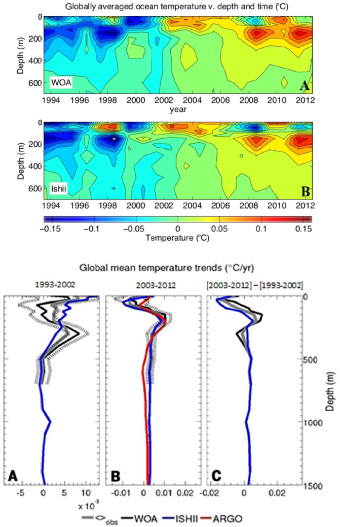
Understanding the various mechanisms involved in the transfer of heat within the climate system was a major focus of the workshop. As much as 93 percent of the heat trapped by greenhouse gases (GHGs) goes into the ocean; the lower atmosphere—where global surface temperature is measured—is a very small heat reservoir in comparison (Rhein et al., 2013). Veronica Nieves of the NASA Jet Propulsion Laboratory presented evidence that during the recent slowdown in GMST rise (in this case, using 2003 as the period start), excess heat was sequestered in the subsurface tropical Pacific waters, which is a “symptom” of decadal variability. In the early 2000s, Pacific surface temperatures were cooler, and unusually strong winds caused the heat to travel to the subsurface (100-300 m) depth layer in the eastern Pacific Ocean to the central/western Pacific Ocean and Indian Ocean. Therefore, as Nieves explained, there was no slowdown in terms of depth-integrated temperature, because when the Pacific Ocean surface gets cold there can be warming beneath and vice versa (global trends shown in Figure 4).
Because water expands as it warms and contracts when it cools, Nieves suggested that global mean sea level may be a more appropriate measure for climate change than GMST because it reflects the depth-integrated ocean heat content.
___________________
1 Empirical Orthogonal Function (EOF) analysis is a method used in statistics and signal processing to decompose a signal or data set in terms of orthogonal (or perpendicular) basis functions that are determined from the data. The EOF method finds patterns in both space and time, although otherwise is the same as performing a principal components analysis on the data. EOF analysis is often used to study possible spatial modes (i. e., patterns) of variability and how they change with time. It is not based on physical processes; rather a field is partitioned into mathematically orthogonal (independent) modes, which sometimes may be interpreted as atmospheric and oceanographic modes (“structures”).
The heat storage of the ocean is much larger than that of the surface layer. Therefore, many participants stressed the importance of understanding the various mechanisms that transport this heat in order to better understand the current state of Earth’s climate and how it changes. This section summarizes the workshop presentations about several of the proposed contributors to and patterns of this heat transport.
Processes and Patterns in the Pacific Ocean
The El Niño–Southern Oscillation (ENSO, see Box 3) is the dominant mode of interannual variability in the Pacific Ocean, with well-known connections worldwide, including to U. S. climate. For example, El Niño (the warm phase of the ENSO) is associated with strong winter effects in the Northern hemisphere that result in more precipitation across the southern United States and cooler than normal temperatures in the southeast, as well as fewer hurricanes (in June to November; Goldenberg et al., 2001). Although the mechanisms surrounding ENSO phases are well studied and understood (see Box 3), the drivers of Pacific Decadal Variability (PDV) patterns are less so, although studies have implicated ENSO as one driver.
Gerald Meehl, National Center for Atmospheric Research (NCAR), emphasized that the precise mechanisms that control decadal variability in the Pacific Ocean and trade winds, including the mechanisms that control phase changes in PDV (i. e., the Pacific Decadal Oscillation [PDO] or the Interdecadal Pacific Oscillation [IPO]), are still a topic of debate. Such phase changes could involve coupled air-sea tropical-mid-latitude processes (Meehl and Hu, 2006) or chaotic (stochastic) amplitude modulation of ENSO (e. g., Jin, 2001), or might be triggered by variability in the Atlantic Ocean (e. g. McGregor et al., 2014; Li et al., 2016).
Importance of the Pacific Ocean to Global Trends
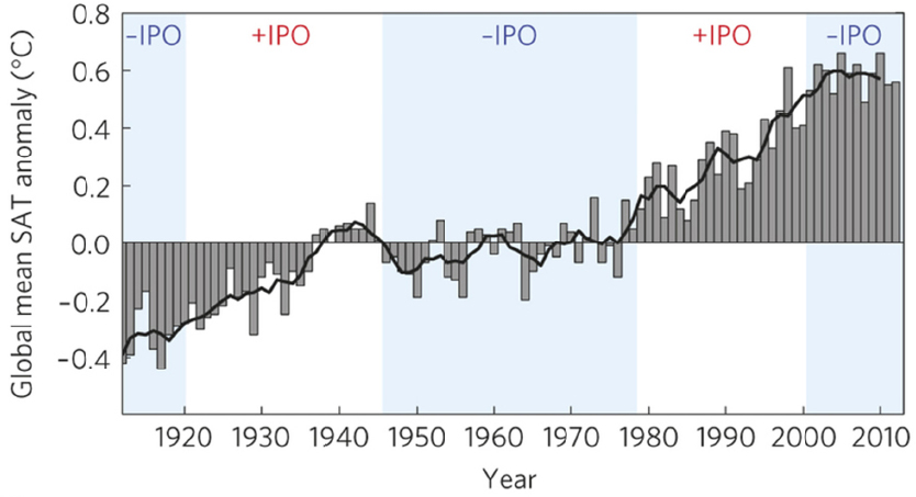
Several participants noted that decadal variability in the Pacific Ocean is a major driver of global variability, which is superimposed on long-term warming trends (Kosaka and Xie, 2013; England et al., 2014; Nieves et al., 2015; Meehl, 2015; Newman et al., 2016). Meehl presented evidence linking phases of the IPO, observed as decadal variability in SSTs across the Pacific Ocean, to decadal variability in GMST. Meehl said the slowdown in GMST in the early 2000s occurred when the IPO was in its negative phase (2000-2013), whereas the IPO was in its positive phase during a previous period of faster warming (late 1970s to late 1990s; see Figure 5). There is also evidence of the influence of PDV in other slowdown periods in the past (e. g., mid-1940s to late 1970s).
The GMST slowdown and the recent negative IPO phase are likely related to the presence of stronger trade winds during the negative phase of the IPO. Stronger trade winds cause a La Niña–like pattern of increased upwelling of cooler waters in the eastern tropical Pacific Ocean and intensified subtropical cell circulation in the atmosphere, which promotes enhanced mixing of warmer water into the subsurface of the ocean. Such enhanced mixing could account for about 50 percent of energy represented in the slowdown in GMST rise (England et al., 2014; Delworth et al., 2015).
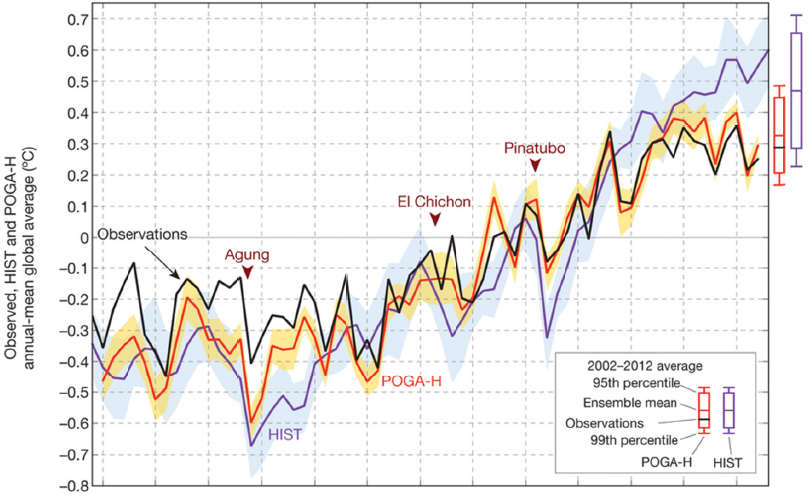
Shang-Ping Xie from the Scripps Institution of Oceanography also presented evidence that the tropical Pacific SST affects timing and magnitude of the warming acceleration and slowdown in GMST, including the recent slowdown period. He presented results from a
POGA (Pacific Ocean-Global Atmosphere) pacemaker2 experiment in which model runs specifying the cycles of internal Pacific variability in SST (from observations) better match observations of GMST than the model runs without Pacific cycles temporally synced to the observations (Figure 6).
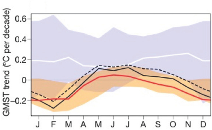
Xie pointed out that GMST, regardless of the robustness of current estimates of this metric, is not measured directly; rather, it represents the average of temperature measured across the globe. Therefore, a lot can be learned about what is driving GMST variability by “unpacking the data” to look for spatial and seasonal patterns. For example, an examination of the slowdown period (in this case, 2002-2012) reveals that colder winter temperatures characterized the slowing trend (Figure 7, January-February-March [JFM] dip). During a Northern Hemisphere winter, storms inject heat from the tropics into the high latitudes; however, during a cold phase of the IPO, the tropics are cooler and transfer less heat. During the summer, the storms do not contribute as much heat to higher latitudes, which allows external forcing (such as GHGs) to dominate the warming trend. Therefore, as Xie explained, wintertime is a distinct seasonal fingerprint of the negative IPO. The pacemaker experiment (POGA-H) also shows the same result.
Mechanisms Driving Pacific Decadal Variability
Antonietta Capotondi of the University of Colorado delved more deeply into the mechanisms that could be driving low-frequency decadal shifts in tropical Pacific climate, ENSO characteristics, and PDV. Several mechanisms for this variability have been
___________________
2 In this context, a “pacemaker experiment” refers to specifying a certain variable (in this case tropical Pacific SST decadal variability) and allowing the free-running coupled model to respond.
proposed. One possible explanation relies on changes in the strength of the wind-driven upper-ocean overturning circulation known as Subtropical-Tropical Cells (STCs). The STCs are characterized by an equatorward subsurface flow, upwelling along the equator, and poleward flow in the thin surface Ekman layer3. Capotondi said that her own studies have shown that the changes in the strength of the STCs are associated with the adjustment of the equatorial thermocline4 to changes in the surface winds (Capotondi et al., 2005).
Capotondi tried to answer the question of which winds were driving the process by studying the abrupt shift in the PDO (an index of PDV, see Box 4) and in the tropical Pacific climate that occurred in 1976-1977, the last time the PDO shifted from a cool to warm phase. Her comparison of wind stresses from the period 1960-1976 to the period 1977-1997 reveals that the biggest differences in wind stress between the two periods are found at 10 S and 13 N. At these latitudes, a large standard deviation of the pycnocline5 depth is associated with enhanced Rossby wave6 activity, which exhibits a pronounced decadal component (Capotondi and Alexander, 2001; Capotondi et al., 2003). Thus, tropical PDV
___________________
3 The Ekman layer is the layer in a fluid where flow results from a balance between pressure gradient, Coriolis and turbulent drag forces. For example, wind blowing North over the surface of water creates a surface stress and a resulting Ekman spiral is found below it.
4 A thermocline is the transition layer between warmer mixed water at the ocean's surface and cooler deep water below.
5 The pycnocline is a boundary layer in the ocean that separates water of differing densities due to temperature or salinity gradients.
6 Rossby waves are a natural phenomenon in the ocean and atmosphere that owe their properties to Earth’s rotation. Oceanic Rossby waves move along the thermocline.
may originate within the tropics and be communicated to the extra-tropics through atmospheric teleconnections via the STCs. However, it is not clear whether changes in equatorial SSTs could feed back into the anomalous tropical winds that drive the STCs, and provide a deterministic mechanism for these tropical decadal climate variations.
An important aspect of tropical PDV is the possible decadal modulation of the interannual ENSO phenomenon. Such decadal modulation may originate from, and/or cause, changes in the tropical Pacific mean state. A study of the changes in ENSO behavior after the 1976-1977 climate shift using Linear Inverse Modeling7 shows that the null hypothesis that those changes are driven by climate noise cannot be rejected (Capotondi and Sardeshmukh, 2016). Thus, tropical PDV, as well as the PDO, may be driven by random system behavior and have limited predictability.
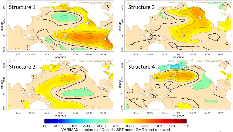
Yochanan Kushnir from Columbia University reminded the audience of the seminal work of Zhang et al. (1997) that discriminated between the patterns of PDV from that of the interannual variability of ENSO. He then discussed recent work by Newman et al. (2016) that suggests that PDV (in this case, the PDO) is likely not a single physical “mode” but rather the arbitrary sum of several different patterns that owe their existence to different dynamical processes. Newman et al. used LIM to separate the North Pacific SST variability
___________________
7 Linear Inverse Modeling (LIM) uses observations to extract the intrinsic linear dynamics that govern the climate. In a LIM model, representations of climate dynamics become more exact as the system becomes more chaotic, whether this chaos arises internally from turbulence or externally from unknown disturbances.
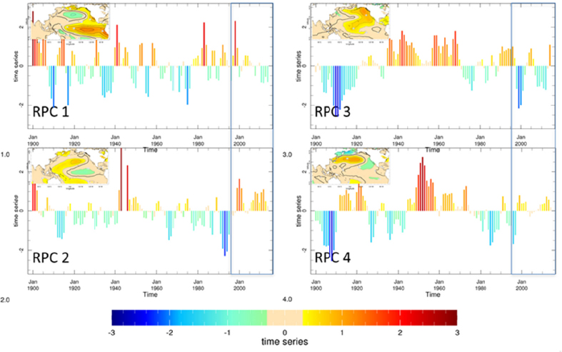
into three distinct basin-wide “dynamical modes,” which closely resemble the leading rotated EOFs (Figure 8). When combining their observed historical intensity and phase relationship (Figure 9), they reproduce the historic record of the PDO.
Examination of the time series of these different patterns over the past century (Figure 9) reveals that they would combine to exhibit a decline in tropical SST at the time of recent GMST warming slowdown. According to Newman et al., the complexity of PDV poses challenges for predictability of the phenomenon, because models would have to achieve the difficult task of capturing the different components of PDV and their governing mechanisms. Similarly, this complexity will hamper representative reconstructions of the PDO using paleoclimate proxies unless the evolution of the different components is captured. Closing gaps in the understanding of these components would involve added observations of the ocean and atmosphere and would improve the ability of coupled models to capture the underlying processes and patterns.
Indian Ocean Variability
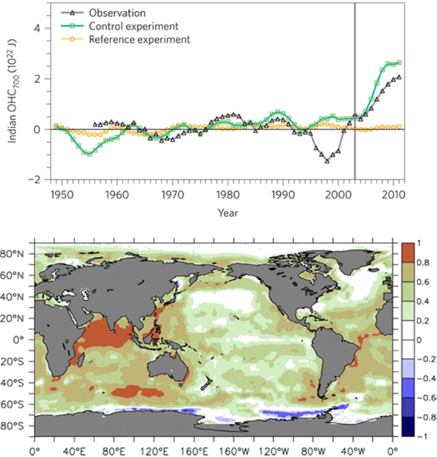
A number of studies reconciled the slowdown in GMST rise and the top of atmosphere (TOA)8 radiation imbalance (which would indicate a warming planet) by an anomalous heat flux into the ocean (e. g., Meehl et al., 2011; Kosaka and Xie, 2013). Those studies indicate a substantial portion of the heat missing from the atmosphere is expected to be stored in the subsurface Pacific Ocean. Veronica Nieves introduced observational evidence of heat storage in the Indo-Pacific region and, to a lesser extent, in the Southern Ocean (Nieves, 2015), as discussed earlier in this chapter. Caroline Ummenhofer from the Woods Hole Oceanographic Institution presented complementary evidence that Indian Ocean variability plays an important role in global ocean heat content and has several important regional climate implications. The Indian Ocean has also been shown to have the strongest correlation between SSTs and GMST since 1900 as compared to other ocean basins (Figure 10, bottom).
Despite this correlation, the Indian Ocean, particularly the western Indian Ocean, has exhibited significant surface warming especially during the last 10 ten years of the recent slowdown (Roxy et al., 2014). This warming is inconsistent with changes in air-sea surface heat fluxes (Yu et al., 2007), suggesting that ocean dynamics play a role in redistributing heat in this region. For example, there is evidence that the subsurface warming in the Indian Ocean has compensated for cooling in the Pacific Ocean via increased heat transport from the Pacific Ocean to the Indian Ocean, carried by the Indonesian Through Flow (Lee et al., 2015; Nieves et al., 2015). As a result, the heat content of the Indian Ocean has increased abruptly (Figure 10, top), which accounts for greater than 70 percent of the global ocean heat gain in the upper 700 m during the past decade (Lee et al., 2015). Nieves et al. (2015) found that warming in the 100-300 m layer of the Indian and Pacific Oceans has compensated for cooling in the top 100 m layer of the Pacific Ocean since 2003. Ummenhofer explained that these recent trends, and the extensive subsurface cooling in the tropical Indian Ocean until the early 2000s, are likely related to multidecadal variations in Pacific wind forcing (Ummenhofer et al., 2016).
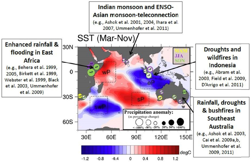
Ummenhofer then discussed how decadal to multi-decadal changes in the upper-ocean properties in the Indian Ocean affect the frequency of Indian Ocean dipole events in different decades. The Indian Ocean dipole is the leading mode of variability in the Indian Ocean and influences regional climate (Figure 11), impacting rainfall and flooding in East Africa; the Indian monsoon and ENSO-Asian monsoon teleconnection; droughts and wildfires in Indonesia; and rainfall, droughts, and bushfires in Southeast Australia.
Decadal Variability in the Atlantic
Atlantic Multidecadal Variability (AMV, also known as the Atlantic Multidecadal Oscillation or AMO, see Box 3) is an index of the swings in the North Atlantic SSTs. The AMV is associated with significant climate impacts both regionally and globally, from northeast Brazilian and African Sahel rainfall (Folland et al., 1986, 2001; Rowell, 2003) to
___________________
8 Together with data derived from ocean heat content increases, radiometers on satellites are used to make TOA measurements of the amount of infrared energy leaving Earth’s atmosphere. This amount is subtracted from the amount of solar radiation entering Earth’s atmosphere to determine Earth’s energy budget—that is, the energy that remains in Earth’s climate system. For Earth’s temperature to be stable over long periods of time, incoming and outgoing energy must be equal—a state referred to as radiative equilibrium or radiative balance. If more energy is leaving than entering, then Earth’s climate will cool. If more energy is entering than leaving, then Earth’s climate will warm. For more information, see Farmer and Cook (2013).
European and North American summer climate (Enfield et al., 2001; McCabe et al., 2004; Sutton and Hodson, 2005). Despite these important impacts, the mechanisms of the AMV are not well understood. Although many studies suggest that the AMV is associated with (or driven by) changes in the Atlantic Meridional Overturning Circulation9 (AMOC)—a zonally integrated representation of Atlantic Ocean circulation (Folland et al., 1986; Gray et al., 1997; Delworth and Mann, 2000; Knight et al., 2005)—other studies suggest aerosols and intrinsic atmospheric variability as possible drivers of the AMV (e. g., Booth et al., 2012; Clement et al., 2015).
Many participants presented on the importance of Pacific variability as a driver for global trends, but there is also work to suggest that Atlantic variability can drive Pacific patterns (Ruprich-Robert, 2016). Other participants presented on mechanisms and drivers of Atlantic variability as well as teleconnections (atmospheric and ocean bridges) between the Atlantic and Pacific basins.
___________________
9 The Atlantic Meridional Overturning Circulation (AMOC) is a major circulation pattern in the Atlantic Ocean that involves the northward flow of warm, salty water in the upper/near-surface layers of the Atlantic Ocean to the North Atlantic and Nordic Seas, and the southward flow at depth of the cold, dense waters formed in those high-latitude regions.
Relationship of the AMOC and the NAO
Some modeling studies suggest that AMOC variability itself is driven by surface buoyancy fluxes associated with the NAO, which is primarily an atmospheric phenomenon that exhibits variability on many timescales, including on decadal timescales (see Box 3). Variability in the NAO has a strong influence on surface climate across the Atlantic basin and beyond (Thompson and Wallace, 2000). Tom Delworth from the NOAA Geophysical Fluid Dynamics Laboratory (GFDL) and Gokhan Danabasoglu from NCAR discussed their work investigating AMOC variability and mechanisms, including related decadal and longer timescale climate variability in the Atlantic, and the role of decadal variability in the NAO.
Delworth highlighted the potential role of the NAO in driving AMOC variability. He presented modeling experiments in which he added heat fluxes to the North Atlantic Ocean associated with the positive phase of the NAO and then examined the resulting response of AMOC and the rest of the climate system (both regionally and globally). His results show that many impacts (e. g., temperature, sea ice extent, and vertical shear of the zonal wind) have larger amplitude at longer timescales because of the role of feedbacks and the time integral of transports. He then applied NAO forcing based on the observed NAO index and concluded that the AMOC response and associated climatic impact depend on the model’s internal AMOC characteristics and mean state. Delworth also showed that models simulate NAO-induced AMOC changes over the historical record consistent with observations of various regions and phenomena: early 20th century warming, cooling in the 1960s-1970s, and warming in the 1980s-1990s of the Subpolar North Atlantic Ocean (70 W-0 W, 30 N-65 N); Arctic sea ice extent; tropical atmospheric circulation; and changes in the Southern Ocean. He concluded that NAO variability drives AMOC variability, particularly on multidecadal scales, although what generates NAO variability on these longer timescales remains unknown.
Because there are no long-term and continuous observations of AMOC and related variables, models remain essential tools for studies of AMOC variability and mechanisms. Danabasoglu presented a systematic assessment of the impacts of several ocean model parameter choices on AMOC characteristics in the Community Earth System Model (CESM, a fully coupled global climate model), with the primary goal of identifying robust and non-robust aspects of AMOC variability mechanisms. Danabasoglu changed some loosely constrained parameter values used in several ocean model subgrid-scale parameterizations, specifically: vertical mixing, submesoscale mixing, mesoscale mixing, and horizontal viscosity parameterizations. He also performed additional sensitivity experiments in which atmospheric initial conditions were perturbed to provide a baseline ensemble set for the parameter sensitivity experiments. He found that both the amplitude and timescale of AMOC variability differ considerably among the simulations, with the dominant timescale of variability ranging from decadal to centennial. Details of how the density anomalies that lead to AMOC changes are derived also differ.
Despite these differences, he noted several important, robust aspects of AMOC variability: (1) the Labrador Sea is the key region with upper-ocean density and boundary layer depth anomalies preceding AMOC anomalies; (2) enhanced Nordic Sea overflow transports do not lead to increased AMOC maximum transports; (3) after AMOC intensification, subsequent weakening is due to advection of positive temperature anomalies into the model’s deep water formation region; and (4) persistent positive NAO anomalies play a significant role in setting up the density anomalies that lead to AMOC intensification via surface buoyancy fluxes.
Effects of the AMV on U. S. Drought
The AMV has been shown to affect the frequency and severity of droughts across North America (Ting et al., 2011). The decadal oscillations in the hydroclimate of the western United States (associated with ENSO) reach extreme severity during the warm and neutral phases of the AMV. For example, the U. S. Great Plains and the Southwest experienced the extremely dry conditions of the Dust Bowl and the persistent Texas drought in the 1930s and the 1950s, respectively. Droughts were less frequent or severe when the AMV was in its cold phase in the early 1900s and from 1965 to 1995.
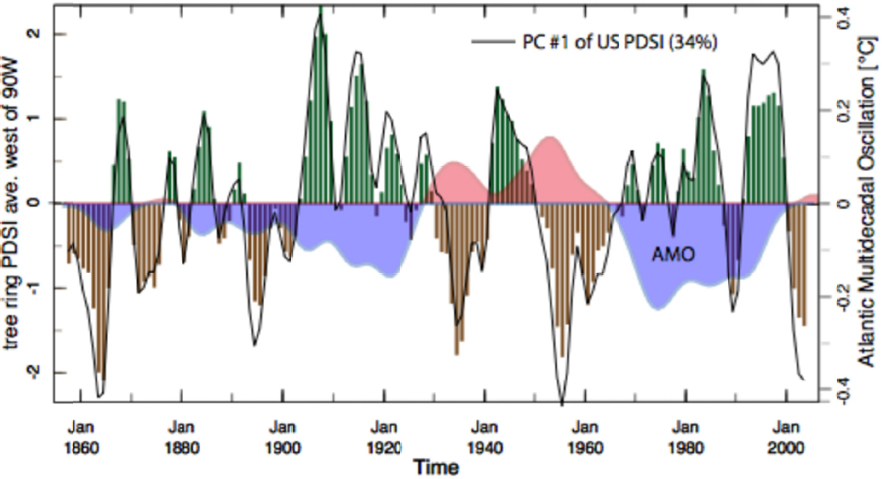
Mingfang Ting of the Lamont-Doherty Earth Observatory of Columbia University said that although the recent U. S. drought is clearly related to the negative phase of the IPO as well as to the global warming trend, the contribution of the AMV may actually be more significant and widespread than is commonly assumed. Longer-term records show a correlation between a negative AMO and positive Palmer Drought Severity Index (PDSI, a measure of drought) in the western United States (Figure 12).
Ting’s work examines the interconnection between the tropical Pacific and tropical Atlantic on decadal timescales, which she said is crucial in realistically representing the hydroclimate impacts of the AMV on North America. She said that many models overestimate the ENSO association with the AMV. Her research shows that models more closely match the observed AMV-North American drought connection when the tropical Pacific SST anomalies associated with the AMV are smaller (< 0.5 degrees). Thus, the observed relationship between warm AMV and dry North America can be severely underestimated in models depending on how decadal tropical Atlantic SST anomalies are
generated in CMIP510 models—whether the relationship is dominated by ENSO conditions in the tropical Pacific or subpolar North Atlantic SST anomalies. Ting said that removing the decadal ENSO impacts on the tropical Atlantic in models produced better agreement between models and observations in terms of atmospheric teleconnections.
Decadal Variability and the Poles
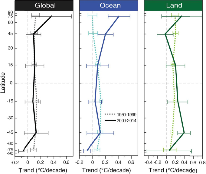
GMST also varies along latitudes on decadal timescales; in particular, there is a pronounced decadal pattern of amplified warming from 2000 to 2014 in the Arctic and slower warming in the Antarctic region (Figure 13). The trends in Antarctic temperature and other associated variables, including sea ice extent, have not been well captured by models, indicating that a better process-level understanding of mechanisms and drivers in that region is needed, according to some participants. In contrast, accelerated warming in the Arctic has been well modeled and observed, highlighting the importance of considering regional variation in surface temperature trends (and data availability with which to calculate trends) and associated regional implications in the context of decadal variability.
Regardless of any slowdown in a globally averaged warming trend, all parts of the Arctic have warmed, which was a topic discussed by James Overland from NOAA’s Pacific Marine Environmental Laboratory. This warming is manifested in loss of snow and
___________________
10 Coupled Model Intercomparison Project (CMIP) phase 5.
approximately 70 percent of sea ice volume over the past century, and does not seem to be associated with any one mode of internal variability.
The warming trend in the Arctic may have an impact on mid-latitude weather and climate variability, but these connections are still controversial (NRC, 2014). The length of the available data series is too short and weather is too chaotic to make a definitive link, said Overland. However, it is understood that as the Arctic warms more quickly, the temperature gradient between the Arctic and the equator is reduced. Overland also said that most researchers think that warming overall will dominate weather patterns, but there will be specific episodic and regional impacts from Arctic warming. Overland showed, as an example of regional impacts, that loss of sea ice in the Kara Sea will weaken winds across East Asia, leading to a strong Siberian High, pushing storms into Japan and China. For more examples, see NRC (2014).
Although the Arctic has been warming and sea ice disappearing, the Southern Ocean has been (mainly) cooling and sea-ice extent has been growing slightly overall. John Marshall, from the Massachusetts Institute of Technology, examined the causes behind such geographic variability and argued that inter-hemispheric asymmetries in the mean ocean circulation (with sinking in the northern North Atlantic and upwelling around Antarctica) strongly influence the SST response to anthropogenic forcing. These asymmetries accelerate warming in the Arctic while delaying it in the Antarctic region. Additionally, while the amplitude of forcing from GHG emissions has been similar at the poles, significant ozone depletion only occurs over Antarctica, he explained.
The initial response of SSTs around Antarctica to ozone-related changes in surface wind trends is cooling, because the Ekman-driven flow in the ocean associated with strengthening westerly winds11 drives cold water equatorward, away from Antarctica. This has potentially influenced the modest increases in sea-ice extents in the Southern Ocean. However, on longer timescales, ozone-induced changes in circulation patterns should result in warmer water being drawn up from below, resulting in warming of SSTs and likely sea-ice decline, explained Marshall.
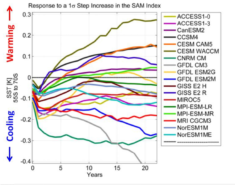
The transition from SST cooling to warming is model dependent. Marshall used models to examine the effects of a step change in wind forcing. He explained that initially models all show cooling, but they respond in different ways over time (Figure 14). A fast response to a wind perturbation (equatorward transport of cooler water) led to cooling, while a slow response led to the upwelling of warmer water and overall warming, which would explain why some models show warming and some show cooling in the region on longer timescales.
What, then, is the mechanism that sets the crossover timescale from cooling to warming? As the wind blows water away from Antarctica, there is a cooling response. However, there is still warm water at depth, so by strengthening the wind, this water comes up from depth to eventually melt the ice, proposed Marshall. The stratification in the Southern Ocean in the seasonal ice zone is set by salinity, being fresh and cold at the surface, warm and salty below. Realistic vertical and horizontal temperature and salinity profiles in the region of seasonal sea-ice are very difficult to capture in models, which could explain why the models display differing behavior. Moreover, the temperature and salinity distributions are not well observed, which highlights the importance of sustaining subsurface observations in the seasonal ice zone, such as the Southern Ocean under-ice Argo program, Marshall concluded.
___________________
11 Winds from the west toward the east in the mid-latitudes (between 30 and 60 degrees).
In summary, basic principles of ocean circulation suggest that one would expect an asymmetric polar response in a warming climate, with accelerated warming in the Arctic and delayed warming in the Antarctic region. In addition, wind-driven changes around Antarctica, due to ozone depletion or natural variability, could account for recent cooling and recent sea-ice expansion, Marshall said. Inter-model differences in the Southern Ocean’s response to wind may be related to different background stratification in the seasonal ice zone. The poles are also not well represented in earlier datasets used for calculating GMST, suggesting that, particularly for the Arctic, GMST trend calculations may be underestimated. Updates in the Karl et al. (2015) analysis include improvements in the representation of the existing Arctic dataset. For further discussion of data needs, see Overcoming Data Limitations.
This page intentionally left blank.


