
4
Implementing Emission Controls on Mobile Sources
INTRODUCTION
Since the earliest days of the Clean Air Act (CAA), mobile sources have been recognized as one of the most important sources of air pollution and, as a result, have been a prime target for emission control. Despite almost three decades of increasingly tight and wide-ranging regulations, emissions from mobile sources are still a major source of air pollution in the United States (see Figure 1-2 in Chapter 1). The persistence of the need to address mobile emissions is not, however, an indication that the largely technological controls applied to mobile sources have been ineffective; indeed, emission rates from individual vehicles have decreased substantially since enactment of the CAA. Instead, human behavior and other social factors, such as increases in vehicle miles traveled (VMT) and the growing popularity of sport utility vehicles (SUVs), which had been regulated at a less stringent level, appear to have offset many of the gains achieved from the imposition of technological controls.1 Difficulties in identifying and repairing high-emitting vehicles was probably also a contributing factor.
Currently, a wide variety of mobile sources are subject to control under the CAA. These are broadly divided into on-road and nonroad sources (see Table 4-1). On-road sources include light-duty vehicles (LDVs, also referred to as passenger cars), light-duty trucks (LDTs), heavy-duty vehicles
TABLE 4-1 Types of Vehicles and Engines Regulated by AQM in the United States
|
Source Category |
Status (Date Promulgated; Effective Date) |
|
On-road sources |
|
|
Light-duty vehicles (LDVs or passenger cars) |
Tier 2 regulations require about 99% reduction over previous control levels for cars (2000; 2004–2007) |
|
Light-duty trucks (LDTs) (pickup trucks, minivans, passenger vans, and sport-utility vehicles with a gross weight of less than 8500 lb) |
Must comply with Tier 2 Lightest truck (2000; 2004–2007) Heavier light trucks (2000; 2008–2009) |
|
Medium-duty passenger vehicles (MDPVs) (vehicles with gross weight 8,500–10,000 used for personal transportation, such as larger sport utility vehicles [SUVs] and passenger vans) |
Tier 2 standards to be phased in beginning with the 2008 model year (2000; 2008–2009) |
|
Heavy-duty vehicles (HDVs) (vehicles with gross weight greater than 8500 lb used commercially, such as large pickups, buses, delivery trucks, recreational vehicles [RVs], and semi-trucks. |
Highway Heavy-Duty Rule requires new vehicles to meet substantially lower PM and NOx standards (>90% reduction) (2001; 2007–2010) Also strict fuel sulfur levels (15 ppm) (2001; 2006) |
|
Motorcycles |
New standards to reduce emissions by 80% (based on California) (proposed 2002; to take effect 2006–2010) |
|
Nonroad Sources |
|
|
Nonroad, spark ignition (gasoline) engines |
For handheld engines, new rules require 70% NOx plus hydrocarbon reduction (2000; 2002–2007) New standards promulgated for larger spark ignition engines (2002; 2004–2007) |
|
Nonroad recreational vehicles and engines |
New rules for variety promulgated to require between 55% and 80% reduction in emissions (depending on pollutant) (2002; 2006–2009, depending on type of engine) |
|
Nonroad compression ignition (diesel) engines |
Nine size ranges, including agricultural and construction equipment; existing rules promulgated in 1998 (1998; 1999–2008) New standards comparable to Highway Heavy Duty Rule proposed 2003 |
|
Source Category |
Status (Date Promulgated; Effective Date) |
|
Marine engines |
New recreational engines required to meet new standards with 55–80% reduction in emissions (depending on pollutant) (2002; 2006–2009) Largest maritime commerce engines regulated to international standards for NOx (not PM) (2003; 2004) Smaller maritime commerce engines regulated for NOx, PM (1999) |
|
Aircraft |
Initial standards for smoke only; new standards adopting International Civil Aviation Organization rules requiring 20% reduction in NOx emissions (1997; full effect in 1999) |
|
Locomotives |
Regulations applying to new locomotive engines and to remanufactured engines from 1973 and later locomotives; ultimately (2040) expected to reduce NOx by 60%; PM by 46% (1997; Tier 0 for engines 1973–2001; Tier 1 for engines 2002–2004; Tier 2 for engines 2005 and later) |
(HDVs), and motorcycles that are used for transportation on the road. On-road vehicles may be fueled with gasoline, diesel fuel, or alternative fuels, such as alcohol or natural gas. Nonroad sources refer to gasoline- and diesel-powered equipment and vehicles operated off-road, ranging in size from small engines used in lawn and garden equipment to locomotive engines and aircraft.
In principle, the mobile-source emissions can be controlled with three types of strategies:
-
New-source certification programs that specify emission standards applicable to new vehicles and motors.
-
In-use technological measures and controls, including specifications on fuel properties; vehicle inspection and maintenance programs; and retrofits to existing vehicles.
-
Nontechnological (for example, behavior modification) measures to control usage or activity (for example, via management of transportation).
This chapter summarizes how each of those strategies is used in the United States and concludes with a critical discussion.
CONTROLLING EMISSIONS THROUGH CERTIFICATION STANDARDS ON NEW VEHICLES AND MOTORS
In the United States, the first mobile-source emission reductions were aimed at lowering the emissions on new vehicles and engines. As older model cars were retired, the in-use fleet would become increasingly populated with regulated vehicles, and emissions would steadily decrease. The first regulations were imposed on passenger cars2 and then were applied to other on-road vehicles, such as trucks and buses, and most recently, to nonroad sources, such as tractors and construction equipment.3,4 The specific emission standards listed in Table 4-1 for mobile-source categories have sometimes been set directly by Congress in an amendment to the CAA, but more typically, the EPA administrator has set such standards. Except for California, states do not have independent authority to set new emission standards (see Box 4-1).
At the same time, as standards have been set for vehicle emissions, vehicle manufacturers have also been required to comply with requirements for Corporate Average Fuel Economy (CAFE) standards, which were initiated by Congress in the Energy Policy and Conservation Act of 1975. CAFE established mandatory fuel efficiencies in the form of required miles per gallon (mpg) goals for fleets of passenger cars and light-duty trucks.5 These standards were enacted in the wake of a petroleum supply interruption and were less concerned with air quality improvements. Nevertheless, for a given vehicle technology, reduced fuel consumption per mile would, in principle, result in lower engine-out emissions, and, therefore, result in less burden on the afterengine emission control system to meet a given emission per mile standard. In practice, implementation of the relatively modest CAFE standards appears to have helped in meeting some hydrocarbon emission standards. However, future application of some especially fuel-efficient engines—which have higher engine-out emissions of some pollutants (for example, NOx)—will likely require development of substantially more effective emission control technologies in order to simultaneously improve fuel economy and emissions (NRC 2002c).
|
2 |
Although the first federal controls on mobile sources began with regulations on passenger cars for the 1968 model year, California began mandating emission controls on passenger cars in the early 1960s. |
|
3 |
An exception is aircraft engines, which have been subject to emission regulations since 1974. The earliest regulations were for smoke from turbojet engines. |
|
4 |
Because nonroad sources have been essentially uncontrolled until recently, their contribution to total mobile-source emissions has grown considerably since passage of the CAA (see Table 4-2). |
|
5 |
The current CAFE program requires vehicle manufacturers to meet a standard in miles per gallon (mpg) for the fleet they produce each year. The standard is 27.5 mpg for automobiles and 20.7 mpg for light-duty trucks. |
|
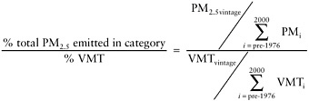
BOX 4-1 The CAA expressly precludes any state except California from setting its own motor vehicle emission standards. Because of California’s experience with the most severe air pollution in the nation, it has historically assumed a leadership role in promoting the application of new control technologies for automobiles. By the 1950s, researchers in California had been able to establish a cause and effect linkage between gaseous emissions from motor vehicles and the formation of photochemical smog with its concomitant high concentrations of O3 and PM. In response to that finding, California enacted legislation in 1961 that established statewide new-vehicle emission standards beginning with the 1966 model year. The federal government followed suit in 1965 with the Motor Vehicle Pollution Control Act, which set similar standards for the entire nation beginning with model year 1968. That pattern has been repeated on numerous occasions, as stricter emission standards have been enacted first in California and then propagated to the entire nation by direct congressional mandate or rule-making by the EPA administrator (see Figure 4-1A,B,C). Although states are not allowed to set their own emission standards, the CAA permits them to choose California’s stricter standards (typically as part of their state implementation plans). In addition to emission standards, states can opt for other aspects of California’s more aggressive program to control mobile-source emissions; these include programs on fuel composition, regulation of individual motorists’ use of their automobiles, and controls on transportation infrastructure planning and investment. As a result, California regulations and programs on mobile emissions have played an important role in state implementation plans throughout the nation (see, for example, the discussion on the Ozone Transport Commission in Chapter 3). |
Emission Standards for Light-Duty Vehicles and Light-Duty Trucks
The CAA Amendments of 1970 required auto manufacturers to reduce LDV and LDT emissions by 90%. That reduction was to be achieved for carbon monoxide and hydrocarbon emissions by 1975 and for nitrogen oxides (NOx) emissions by 1976 (Jacoby et al. 1973). However, these standards were not fully implemented until the 1980s. Claiming that the initial compliance dates for a 90% reduction in LDV and LDT emissions were infeasible, the auto industry achieved only a partial implementation of the mandated emission-reduction goals by 1975–1976 (Howitt and Altshuler 1999). The CAA Amendments of 1977, extended the emission standards deadlines for carbon monoxide and hydrogen until 1983 and 1980, respectively. The amendments also extended the deadlines for NOx to 1982 and changed the standard from a 90% to a 75% reduction. In addition, the amendments allowed the EPA administrator to relax the NOx requirement selectively until 1984 for automotive technologies that promised better fuel economy (Crandall et al. 1986).
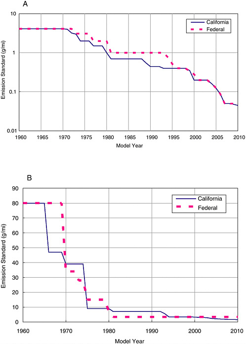
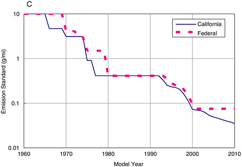
FIGURE 4-1 The evolution of California and federal tailpipe standards on passenger car exhaust emissions since the 1960s. (A) NOx emissions, (B) CO emissions, and (C) VOC emissions. NOTE: A, B, and C are not completely consistent. There have been changes in test methods that are accounted for in an approximate manner. Current emission standards for VOC are defined in terms of nonmethane organic gases (NMOG). In addition, the most recent emission standards are based on vehicle categories and an average over these categories. For the California program, manufacturers must meet a fleet average standard for NMOG; for the federal program, manufacturers must meet a fleet average standard for NOx. The “standards” for CO and NOx in California for 1999 and later and the federal standards for NMOG and CO in model years 2004 and later are based on an assumed distribution of standards used for compliance. In addition, vehicles currently have to meet additional useful life standards and standards for supplemental test procedures to test operation under off-cycle driving conditions and under airconditioning operations. Thus, the actual progression of standards has been more stringent than shown in the figure. These figures are for exhaust emissions only. For the uncontrolled vehicles in 1960, there were also VOC emissions from crankcase blowby, which have been completely eliminated, and evaporative VOC emissions, which have also had a high degree of control. Note that the vertical axis on the VOC and NOx charts is a log scale. The federal Tier II standards apply to a full useful life of 120,000 miles. Those standards have been adjusted to equivalent 50,000-mile-useful-life standards using data from CARB, which has standards for both 50,000 and 120,000 miles.
Despite the difficulties and delays in implementation, passage of the emission standards from LDVs and LDTs represented a watershed in AQM in the United States: Congress’s adoption of a “technology-promoting” strategy for lowering mobile-source emissions and, over time, industry’s response by developing and installing new and innovative pollution-control technologies for passenger cars (for example, catalytic converters) (see Box 4-2). As this new technology was developed, refined, and installed on new LDVs and LDTs in the 1980s, the emission characteristics of new vehicles sold in the United States steadily and dramatically improved. As higher-polluting vehicles were replaced by newer ones, emission controls became widespread in the U.S. automotive fleet (Howitt and Altshuler 1999). The catalytic-control technology developed in the United States to meet the emission standards mandated in the CAA is now broadly used throughout the world. In China, for example, all cars operated in the Beijing metropolitan area are required to have catalytic controls either as factory-installed equipment or as a retrofit (Liu et al. 1999; Webb 2001).
Despite those technological advances, many areas could not meet the National Ambient Air Quality Standards (NAAQS) for ozone (O3). That was due to challenges in reducing emissions from all sources, but among mobile sources, there was continued growth in VMT and new scientific and technological information that some emissions, especially evaporative emis-
|
BOX 4-2 The development and widespread application of pollution-control technologies have permitted reductions in criteria pollutant emissions even while vehicle miles traveled has continually increased. Early pollution-control technologies included positive crankcase ventilation valves to direct crankcase blowby emissions into the engine; charcoal canisters to sequester volatile hydrocarbons for later burning in the engine, exhaust gas recirculation valves to reduce NOx formation during fuel combustion; and catalytic converters designed to oxidize partially combusted hydrocarbons and CO to CO2. Today, vehicles are being driven by cleaner fuels (for example, the removal of fuel sulfur to extend the life of catalytic converters and the further development and improvement of emission-control technologies including high-performance and three-way catalytic converters capable of reducing NOx to nitrogen gas, hydrocarbon adsorbents, coupled engine-exhaust controls that optimize air-to-fuel mixtures, and leak-free exhaust systems). These technologies are also being expanded for use on heavy-duty vehicles and nonroad equipment. The recent introduction of new automotive technologies, such as electric-gasoline hybrid vehicles with lower fuel consumption, will further decrease emission levels. The continued development of new technologies and application of current technologies to unregulated or less stringently regulated sources is expected to continue to drive decreases in criteria pollutant emissions. |
sions, were not being fully controlled. In addition, HDVs and nonroad vehicles were important contributors. The CAA Amendments of 1990 mandated emission reductions (referred to as Tier I controls) for LDVs by 1994. In addition to calling for further reductions in NOx and volatile organic compounds (VOCs), the 1990 requirements tightened significantly the controls on evaporative emissions, especially during refueling.6 Also, the 1990 CAA Amendments authorized the EPA administrator to establish more stringent Tier II controls in 2004 if they were judged to be needed, technically feasible, and cost-effective (Howitt and Altshuler 1999). The Tier II regulations have since been promulgated. Besides the tightening of NOx and VOC emission standards, Tier II includes a limit on the sulfur content of fuels (to extend the effective lifetime of catalytic converters) and regulations on medium-duty passenger vehicles (MDPVs), such as the largest SUVs,7 as well as a provision that allows manufacturers to use fleet averaging to meet the NOx standards. The entire set of regulations will be phased in between 2004 and 2009.
The CAA authorizes California to set stricter vehicle emission standards because of the magnitude of its air pollution problems. California required manufacturers to achieve average emissions that were lower than those mandated by the federal Tier I regulations, beginning with the 1994 model year. The state also defined a family of low-emissions vehicles: the transitional low-emissions vehicle (TLEV), the low-emissions vehicle (LEV), and the ultra-low-emissions vehicle (ULEV). In addition, California required manufacturers to offer consumers so-called zero-emission vehicles, or ZEVs,8 by 1998 and achieve a 10% statewide market share for ZEVs by 2003 (Sperling 1991). California has delayed and modified its requirement for ZEVs and has recently made additional modifications in response to a June 2002 federal district court injunction that prohibits implementation of
the 2001 Amendments to the ZEV program for the 2002 and 2003 model years.9
The CAA authorized states other than California to adopt the California standards. After the 1990 CAA Amendments set more stringent requirements for nonattainment areas, Maine, Massachusetts, New York, and Vermont chose to include California mobile emission standards in their state implementation plans (SIPs). In 1994, the Ozone Transport Commission (OTC) (described in Chapter 3) petitioned EPA to impose these automotive technology standards on the entire region, including the states that had not done so individually (Howitt and Altshuler 1999). EPA complied, but their decision was overturned when the District of Columbia circuit court determined that EPA lacked the authority to do so.
A series of negotiations among concerned states, automobile manufacturers, environmental groups, and EPA that took place between 1995 and 1998 led to the national low-emission vehicle (NLEV) program. EPA set regulations for this voluntary program; these regulations came into effect only when individual states and automobile manufacturers opted into the program. ZEVs, and the ability of individual states to require them by electing to apply California vehicle standards, were a major issue in these negotiations. Ultimately, Massachusetts, New York, and Vermont retained the requirement for California vehicles, including ZEVs, while the NLEV program was applied in all other states.
With the implementation of the Tier II program, the difference in standards between the California program and the federal program will be substantially reduced, one exception being the ZEV mandate in California, Massachusetts, New York, and Vermont.
Emission Standards for Heavy-Duty Vehicles
LDVs have traditionally been the target of new-vehicle emission standards. However, as emission rates from LDVs declined and the use of on-road freight increased, HDVs became responsible for an increasing fraction of the overall mobile-source emissions of NOx and particulate matter of up to 10 micrometers in diameter (PM10) (EPA 2001a, 2003a). The differentiation between LDVs and HDVs historically has been 8,500 pounds gross vehicle weight (the weight of the vehicle plus the weight of the rated load-hauling capacity). In response to this trend, EPA began regulating HDVs in the 1980s and adopted new-vehicle emission standards at several junctures.
EPA issued new, even more stringent regulations on emissions from HDVs in early 2001 (65 Fed. Reg. 59896 [2000]; 66 Fed. Reg. 1535 [2001]). These new regulations are similar to the Tier 2 standards for LDVs discussed in the previous section in that they require both a tightening of emission certification standards and a decrease in the fuel sulfur content. The regulations, to be phased in between model years 2004 and 2010, will reduce PM and NOx emissions by at least 90% from current standards. To meet these more stringent standards for diesel engines, the sulfur content of diesel fuel will be reduced by 97% from its current level of 500 parts per million (ppm) to 15 ppm beginning in 2006 in most cases.
The HDV emission standards are technology-promoting in that they will require the use of new exhaust-after-treatment technologies for diesel-powered HDVs, as well as substantial requirements for control technology life (up to 435,000 miles in some vehicles). In contrast to LDVs, which have included after-treatment technologies (catalytic converters) since the mid-1970s, previous emission standards on HDVs have only required modifications of engine operations. However, meeting the new NOx and PM standards will require diesel-powered HDVs to further refine engine operations, as well as include control technology for NOx and PM.
Emission Standards for Nonroad Engines
Compared with the long history of regulation of LDV emissions, nonroad mobile-source emissions, like HDV emissions, have been relatively unregulated and, as a result, represent a growing fraction of overall mobile-source emissions (see Table 4-2). In fact, with the set of currently enacted controls, nonroad emissions already exceed on-road emissions of PM and are projected to exceed on-road mobile emissions of VOC and carbon monoxide (CO) in the next two decades. Regulation of these emissions presents some specific challenges to air quality management (AQM). For
TABLE 4-2 Contribution of Nonroad Emissions to Mobile-Source Total and to Manmade Total
|
|
Nonroad Emissions (1,000s of tons per year), yr |
Nonroad as a Percent of Mobile-Source Total, yr |
Nonroad as a Percent of Manmade Total, yr |
|||
|
Pollutant |
2000 |
2020 |
2000 |
2020 |
2000 |
2020 |
|
HC |
3,488 |
3,139 |
47.7 |
58.0 |
19.1 |
20.3 |
|
CO |
25,843 |
37,331 |
34.2 |
43.3 |
26.4 |
34.0 |
|
NOx |
5,447 |
4,164 |
40.6 |
67.0 |
22.2 |
25.7 |
|
PM |
466 |
510 |
66.0 |
77.9 |
15.0 |
16.8 |
|
SOURCE: EPA 2002r. |
||||||
example, nonroad emissions are emitted from a wide variety of engines, including land-based diesel engines (tractors, backhoes, and generators), land-based spark ignition engines (chain saws, lawn mowers, airport ground-service equipment, and motorcycles), marine engines, jet and propeller aircraft engines, and diesel locomotives. In most cases, individual emission-control strategies need to be devised for each engine type and for widely varying use and performance cycles.10 Although control of many new nonroad engines, such as portable power equipment and construction vehicles, can follow implementation and jurisdiction patterns similar to those used for on-road vehicles, the control of substantial emissions from aircraft and engines used in international maritime commerce is made much more difficult by the diverse international jurisdictions under which these vehicles fall.
The 1990 CAA Amendments directed EPA to prepare a study of the scope and sources of nonroad emissions and to regulate them if they were found to make a substantial contribution to O3 or CO nonattainment. The EPA report did not make a formal determination of a significant effect, but it contained an inventory of emissions from nonroad sources and concluded, “because nonroad sources are among the few remaining uncontrolled sources of pollution, their emissions appear large in comparison to the emissions from sources that are already subject to substantial emission-control requirements” (EPA 1991). EPA regulations for some of these engines and vehicles started in 1995, and subsequent regulations continue to bring new classes of engines and vehicles under regulation while more stringent regulations are being prepared to replace existing control requirements. In 2002, EPA finalized regulations for a number of nonroad engines and vehicles, including large spark-ignition engines and recreational vehicles (67 Fed. Reg. 68242 [2002]). In April 2003, the agency proposed a national program to reduce emissions from nonroad diesel engines by combining engine and fuel controls. It is expected that engine manufacturers will meet proposed emission standards by producing new engines with advanced emission-control technologies. Because these control devices can be damaged by sulfur, EPA is also proposing to reduce the allowable level of sulfur in nonroad diesel fuel. The proposed exhaust emission standards would apply to diesel engines used in most kinds of construction, agricultural, and industrial equipment and are expected to reduce emissions by
greater than 90% as compared with today’s engines. The proposed standards would take effect for new engines starting as early as 2008 and be fully phased in by 2014. The regulations plan to lower sulfur concentrations in diesel fuel from the current uncontrolled level of 3,400 ppm to 500 ppm beginning in 2007 and then to 15 ppm in 2010 (EPA 2003i; 68 Fed. Reg. 28328 [2003]).
Control of Mobile-Source Air Toxic Emissions
According to the 1996 National Toxics Inventory (NTI), major stationary sources account for approximately 25% of hazardous air pollutant (HAP) emissions, mobile sources contribute 50%, and area sources (for example, commercial dry cleaning facilities) and miscellaneous sources contribute the remaining 25% (EPA 2001a).
Section 202 (l) of the CAA required EPA to study emissions of air toxics from mobile sources and fuels and set standards for benzene and formaldehyde at least. EPA issued a first draft of the study in 1993. The agency’s final rule on control of emissions of air toxics from mobile sources, incorporating the final version of the study, was issued in March 2001 (66 Fed. Reg. 17230 [2001]). The rule was issued in accordance with a judicial consent order that mandated EPA action once it had missed the CAA deadline.
The rule identifies 21 air toxics associated with mobile sources (including nonroad mobile sources as well as LDVs and HDVs). The agency projects that existing tailpipe, evaporative, and fuel formulation regulations on vehicles and fuels will reduce emissions of benzene, acetaldehyde, and formaldehyde by approximately 70% in 2020 as compared with 1990 levels and that emissions of diesel PM from on-road vehicles will be reduced by 90% (EPA 2000d). The rule requires gasoline refineries to maintain their average 1998–2000 levels of toxic-emission control in response to existing toxic-emission performance standards for reformulated gasoline (RFG) and gasoline. Because of the substantial progress projected from the other emission-control standards and from those soon to be promulgated (as discussed previously in the chapter), no other new standards are set for either vehicles or fuels. A lawsuit contending that the rule is inadequate was filed against EPA on May 24, 2001, by the attorneys general of New York and Connecticut and a consortium of environmental groups.
Implementation of Emission Standards for New Mobile Sources
Motor-vehicle emission standards are implemented through a certification procedure in which manufacturers provide EPA or the California Air Resources Board (CARB) with prototype data showing that the vehicles
meet the emission standards for the legally mandated vehicle lifetime. Following a satisfactory agency review of these data, the manufacturer is issued a certificate of compliance, which allows the production of vehicles to proceed. Produced vehicles are then tested to ensure that the new vehicles meet the applicable emission standards. In addition, in-use vehicles are tested to ensure that the vehicles maintain their performance over time. A failure to maintain in-use performance can result in a recall. Manufacturers are also required to provide a warranty on the emission controls in the vehicle.
The initial exhaust-emission test used to certify cars, referred to as the federal test procedure (FTP), was based on measurements that sought to replicate driving during a typical vehicle trip in downtown Los Angeles during the 1960s. In this procedure (known as a test cycle), the vehicle exhaust is continuously collected and quantified as the vehicle is started and run through a series of operating modes (for example, cold start, accelerations, and decelerations). However, the FTP had a number of shortcomings when it was used to forecast in-use mobile emissions: (1) driving behavior and conditions vary so widely that it is difficult to represent all; (2) because of limitations in the dynamometers used at the time the test procedure was developed, the maximum acceleration during the test had to be limited unrealistically to 3.3 miles per hour per second (mph/sec); and (3) most of the vehicle speeds in the FTP are below 30 mph, a speed that is not reflective of the actual speeds used by most motorists in the United States. Thus, “off-cycle” emissions occurred during vehicle-operating modes that were not tested in the FTP. Although vehicles were certified to appropriate standards, their real-world emissions were higher than would be expected by the standards.
Congress sought to remedy the off-cycle emissions problem in the 1990 CAA Amendments by requiring EPA to control off-cycle emissions. To do so, EPA developed the supplemental federal test procedure (SFTP), which tests cars over an extended range of speeds and accelerations. Certification to the SFTP will be fully phased in by the 2004 model year. However, questions persist whether the SFTP fully captures the large increases in emissions that occur due to rapid accelerations and other changes in the vehicle load.
In addition, EPA took steps to address the issue of evaporative emissions. The test cycle for evaporative emissions was originally developed around 1970, and initial controls on evaporative emissions used a test procedure to measure emissions that would occur from a parked car (called diurnal emissions) and from a car that had just ceased operation (called hot-soak emissions). Like FTP for exhaust emission, these tests proved to be poor predictors of actual mobile evaporative emissions. Between 1987 and 1993, EPA developed a new test procedure for evaporative emissions
that measured evaporative emissions under a more demanding set of operating conditions.11 Under the test procedure (59 Fed. Reg. 16262 [1994]), evaporative emissions are collected by placing a vehicle in an air-tight enclosure and measuring the released hydrocarbons. The test is called the sealed housing evaporative determination (SHED) test. Under this test, the activated carbon canister that traps evaporative emissions vented from the tank is initially loaded with fuel vapor. That is followed by a period of driving that purges the fuel vapor from the canister and into the engine. Next, emissions are measured from a parked car during a simulation of repeated hot days. Finally, evaporative emissions are measured during vehicle operation to assess running losses.
In addition to controlling evaporative emissions vented from the vehicle fuel tank via onboard refueling vapor recovery (ORVR) controls, EPA regulations also require gasoline-filling stations to recover gasoline vapors emitted from filler pipe during refueling operations using so-called stage-two systems.12 California, per that state’s stationary-source regulations, has used these systems to control refueling emissions since the late 1970s. The 1990 CAA Amendments required stage-two systems in all except marginal O3 nonattainment areas. There is a possibility that stage-two and ORVR controls can interact to reduce the effectiveness of both. Because the ORVR system removes fuel vapors displaced from a tank during refueling, the stage-two system would force air, rather than fuel vapors, into the underground gasoline storage tanks, potentially leading to increased gasoline evaporation and fugitive vent emissions. CARB initially considered seeking a waiver from ORVR regulations for California vehicles, but later adopted ORVR systems to promote a consistent vehicle design for all 50 states and to reduce the testing burden for vehicle manufacturers. CARB has since promulgated regulations for enhanced stage-two vapor recovery, which includes measures to ensure compatibility with ORVR systems. The on-board recovery systems were phased in on passenger cars between 1998 and 2000; they will be phased in on LDTs between 2001 and 2006. After these systems are in widespread use (probably sometime after 2010), EPA intends to drop the requirement for stage-two systems (EPA 1998d).
Emissions control for HDVs applies emission standards to the engines, which are tested on an engine dynamometer before being installed in the HDV. The test cycle is based on engine torque and rotational speed. The emission standards are written in terms of the emission rate per unit power
output, typically in grams per brake horsepower-hour (g/bhp-hr) or grams per kilowatt-hour (g/kW-hr).
CONTROLLING IN-USE MOTOR-VEHICLE EMISSIONS
Light-Duty Vehicle and Truck Emissions Inspection and Maintenance Programs
Characterizing emissions from in-use mobile sources has long been a controversial issue. Emission measurements in the field have shown that vehicles in use sometimes do not perform as well as those tested by the manufacturers during certification. High-emitting vehicles (commonly referred to as high emitters) appear to be a major factor. A small fraction of the fleet of LDVs and LDTs in the United States are responsible for a disproportionately large fraction of the total mobile-source emissions (NRC 1991, 1999b, 2001c; Holmes and Cicerone 2002). In some cases, the high emitters have very high evaporative emissions, most likely because of leaks in the fuel system and, in other cases, high tailpipe emissions, due to faulty emission-control systems, or poor engine maintenance.
The initial response to these problems was the development of inspection and maintenance (I/M) programs. In implementing the 1977 CAA Amendments, EPA determined that many states needed annual or biennial I/M programs to ensure that the tailpipe emission-control devices it had mandated were in place and operating properly. In some cases, motorists appeared to intentionally disable these devices or damage them by using leaded gasoline (Howitt and Altshuler 1999). Even though I/M programs did not affect everyday travel behavior and could often be combined with vehicle-safety inspections already required by some state and local authorities, a number of states adopted programs only when the federal government invoked sanctions authorized in the CAA and suspended much of their highway funding (Howitt and Altshuler 1999).
The 1990 CAA Amendments strengthened EPA’s position with regard to I/M by specifically mandating enhanced I/M programs in a number of nonattainment areas. In response, EPA developed an enhanced I/M program with dynamometer testing by using a special cycle known as IM240.13 Although the enhanced I/M requirements in principle allowed states a choice for their program, the requirements in the 1990 Amendments and the stringent criteria that EPA developed for program effectiveness gave states little choice but to accept EPA’s version. For example, EPA’s model (MOBILE)
for estimating emission-reduction benefits from I/M for SIP development greatly discounted benefits from programs that did not meet the EPA criteria. As a result, implementation of enhanced I/M has been highly contentious, with California and, to a lesser degree, other states fighting to implement alternative plans (see, for example, IMRC 1995a,b). In response to the controversy, Congress provided states with greater latitude in a provision of the 1995 National Highway System Designation Act (Bennett 1996). Most states subject to the requirement are currently proceeding with some form of enhanced I/M, but few have been willing to adopt the full set of practices that EPA prescribed in its original enhanced I/M regulations (Howitt and Altshuler 1999).
In addition to the political and regulatory controversies associated with I/M, serious technical questions persist. Recent scientific and technical reviews of I/M have concluded that these programs have been less effective than originally forecasted in identifying vehicles with faulty and/or noncompliant emission-control devices (NRC 2001c; Holmes and Cicerone 2002). Thus, there is a continuing need for an effective regulatory program that can identify and then facilitate the repair or removal of high-emitting vehicles from the fleet (NRC 2001c). It is possible that tailpipe testing programs will be eventually supplanted by other more effective mechanisms for ensuring in-use compliance with vehicle emission standards. First, the in-use performance of 1990 and later model-year vehicles appears to have been significantly better than that of vehicles of earlier model years, perhaps because of the maturing of emission-control technology and the requirements for extended warranties. Second, remote-sensing technologies (see discussion below) are becoming increasingly sophisticated and could provide accurate measurements of in-use vehicle emissions under actual driving conditions. Finally, on-board diagnostic (OBD) systems,14 specifically the OBDII system which has been required on vehicles since 1996, periodically check many emission-control functions (with oxygen sensors, for example). If a problem is detected that could cause emissions to exceed 1.5 times the emission standards, the OBDII system illuminates a malfunction indicator light, known as the “check engine” light on vehicle dashboards. However, broad implementation of OBD in state I/M programs is still in early stages. Because the real-world effectiveness of OBDII in I/M programs has not yet been demonstrated, the transition from direct tailpipe measurement to reliance on these alternative procedures in I/M programs should proceed cautiously, retaining levels of direct tailpipe measurement to confirm that such systems are functioning effectively. Further, it remains
to be seen whether those procedures will be acceptable to the American public.
Remote Sensing of In-Use Vehicle Emissions
A few states have adopted I/M programs that assign a supplementary role to on-road emissions testing by using remote-sensing technology (TNRCC 2003a; Fresno Bee 2002; Laris 2002). In some states (for example, Texas), roadside enforcement officers use remote sensors to identify vehicles that have malfunctioning emission-control systems (similar to the way officers use radar to identify vehicles exceeding the speed limit) and then record license plate numbers. The owners of the vehicles can then be contacted and required to take appropriate corrective actions. Other states, such as Colorado and Missouri, use a “clean screening” program, in which roadside remote sensing is used to exempt vehicles from central testing requirements.
In principle, the use of remote sensing has a number of advantages over a test-center-based inspection system. Remote sensing provides a method for identifying certain types of high tailpipe emitters that periodic inspection at a test facility using a test cycle might not capture; it also can identify high-emitting vehicles that are not showing up for testing (NRC 2001c). At the same time, challenges remain for remote sensing. First, further controlled testing of the technology for quality assurance and quality control, as well as development of technologies for other mobile-source pollutants, such as PM, will be important to its expanded use. In addition, because remote sensing does not monitor a vehicle over its full range of operating conditions and is not yet able to monitor evaporative emissions, it is probably best used at this time as an adjunct to annual or biennial inspections and on-board diagnostics. Other technical issues include site selection of the sensing equipment and the effect of weather conditions on the equipment.
In-Use Emissions from Heavy-Duty Vehicles and Engines
Ensuring that in-use emissions of HDVs (both on-road and nonroad) meet intended standards is considerably more challenging than it is for LDVs and LDTs. First, the durability of HDVs (Davis and Diegel 2002), and the large initial capital investment to replace them, means that older vehicles and engines remain in service much longer, delaying the benefits expected from the introduction of newer, cleaner vehicles and engines (see Box 4-3). Second, it is difficult to conduct in-use emissions testing for HDVs; unlike cars, they cannot be simply placed on a dynamometer to check their emissions through a full driving cycle. Although a number of states have implemented “smoke” regulations that remove gross diesel emit-
|
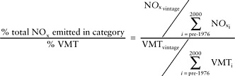
BOX 4-3 Emissions from HDVs are substantially higher in older models than in newer models. Table 4-3A and 4-3B shows the average PM and NOx emissions for HDVs by model year from pre-1976 to 1976 through 2000 and the percent total PM2.5 and NOx emitted in each category for the percent of vehicle miles traveled (VMT). Emissions were calculated for the national fleet traveling on U.S. freeways in July 2000. The three classes of trucks make up most of the heavy-duty fleet. Substantial decreases in PM emissions have been obtained with newer vehicles. Diesel trucks built before 1980 emit 10 times the PM emissions in grams per mile than do trucks built after 1996. The higher ratios of percent total PM emitted in category to percent VMT indicate that older trucks generally are substantial PM emitters despite being used less than newer trucks. Although trucks built before 1981 represent only 4% of VMT, they are responsible for about 11% of the PM emissions from trucks. NOx emissions have not shown as large a decrease because hydrocarbon and CO standards that went into effect during the 25-year period increased combustion temperatures, resulting in increased NOx emissions. In addition, the use of NOx “defeat devices”a has resulted in an increase in NOx emissions in newer trucks. However, diesel trucks built before 1977 emit twice as much NOx as those built after 1996, and those built between 1977 and 1980 emit 50% more than those built after 1996. NOx emissions from trucks built before 1981 represent about 5% of the total from trucks. |
ters from the highway, they are only sporadically enforced in some states, and do not necessarily identify the emitters of high concentrations of fine particles and NOx, which cannot be correlated with smoke. As a result, a large number of older high-emitting vehicles remain on the road, especially for short-haul service in urban areas where the greatest population exposures can occur. A 1997 census of truck use in the United States (DOC 1999) showed that, although most trucks are used for local trips (less than 50 miles/day), the newest trucks tend to be used for the longest trips (Figure 4-2). Some states (for example, California, replacing public school buses) and recently EPA have initiated programs to accelerate the replacement and retrofit of older vehicles, but to date these programs have not been systematic and have relied to some extent on the availability of state funds, which in the current economy have become increasingly scarce.
Perhaps even more challenging is the evidence that at least some of the newer, purportedly cleaner vehicles were operating with emissions in excess of the standards for which they were certified. In 1998, EPA undertook enforcement actions against six diesel engine companies for producing ve-
TABLE 4-3A Average PM2.5 Emissions by Vehicle Model Years for Medium- and Heavy-Duty Trucks
hicles that operate to maximize fuel economy in a way that resulted in unacceptably higher NOx emissions (63 Fed. Reg. 59330 [1998]). EPA also initiated more procedures for in-use testing, and the 2007 rules, discussed earlier in this chapter, have substantially increased durability requirements for control systems—to as much as 435,000 miles (66 Fed. Reg. 5002 [2001]).
TABLE 4-3B Average NOx Emissions by Vehicle Model Years for
Regulating the Content of Gasoline and Diesel Fuels
For most of the first 20 years of implementing the CAA, mobile-source emissions were controlled through technological changes to engines and exhaust systems. With the exception of lead (see Box 4-4), fuel was not
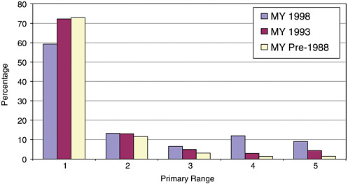
FIGURE 4-2 Percentages of U.S. trucks within selected model years (MY) used for various primary daily driving ranges: (1) up to 50 miles, (2) 51 to 100 miles, (3) 101 to 200 miles, (4) 201 to 500 miles, and (5) more than 500 miles. The survey includes light-, medium-, and heavy-duty trucks. The survey excludes vehicles owned by federal, state, and local governments; ambulances; buses; motor homes; and farm tractors. SOURCE: Data from DOC 1999.
regulated for emissions control. Beginning in the late 1980s, however, a more balanced strategy began to take shape that combined regulations on vehicle performance with regulations on the fuels used by those vehicles (see Table 4-4). This strategy was driven by a desire to control emissions from the entire vehicle fleet—both old and new vehicles—at one time and by emerging control technologies that were especially sensitive to some fuel elements (especially sulfur). The result has been a number of regulations that control fuel content and formulation by EPA under the CAA, as well as by states.
In addition to these regulations, there have been various proposals and requirements in the CAA, state rules, and national energy legislation for the promotion of alternative fuels to reduce the emissions from motor vehicles. Fuels proposed for this purpose include methanol, ethanol, natural gas, liquefied petroleum gas (LPG), and hydrogen. Although these fuels have some limited use, fuel and distribution infrastructure costs have prevented their widespread adoption. Electric vehicles using batteries or fuel cells have also been required or promoted. Current battery technology provides vehicles with limited range, and although they have been introduced into the market, they have not been received well. Vehicle manufacturers are hoping to introduce a limited number of fuel-cell vehicles over the next
|
BOX 4-4 Most of the federal regulations on gasoline aimed at improving air quality were implemented following the CAA Amendments of 1990. One notable exception is the requirement in the 1970s to remove tetraethyl lead from fuels, an action that led to one of the best documented benefits to human health from AQM in the United States through an innovative market-based approach that allowed petroleum refineries to trade and bank lead-reduction credits to lower implementation costs (see Chapter 5). As a result of the removal of lead from gasoline, the concentration of lead in the atmosphere dropped precipitously, and that in turn resulted in a very significant and measurable decrease in blood concentrations in Americans. It is estimated that the drop in blood concentrations in children (see Figure 4-3) has resulted in 30,000–60,000 fewer individuals with IQs below 70 each year (EPA 1997). However, the decrease in blood concentrations was not the primary rationale for the decision to phase out lead in gasoline. This decision was precipitated by the requirement for catalytic controls on LDVs and LDTs to meet the emission standards mandated in the 1970 CAA Amendments. Because lead contaminates metal catalysts, rendering them permanently ineffective, lead had to be phased out of gasoline. As a result of the lead phase-out and introduction of catalytic controls, substantial reduction in pollutant emissions from LDVs and LDTs was achieved. There was also an unintended negative consequence of the lead phase-out. Tetraethyl lead was originally introduced into gasoline as an octane enhancer to improve vehicle performance. To maintain octane levels after the phase-out of lead, refiners blended higher amounts of light hydrocarbons and aromatics, such as benzene, into the fuel. The blending had the unintended consequence of increasing evaporative VOCs and air toxic emissions (EPA 1973; Johnson 1988; NRC 1991).a At the same time, one of the responses to replacing lead, especially in premium gasoline, was the beginning of the use of small quantities of MTBE. The requirements in the 1990 CAA Amendments to control evaporative emissions from LDVs and implement the reformulated gasoline program were in large part an effort to reverse the increase in evaporative VOCs. The 1990 Amendments also required a substantial increase in oxygen content, resulting in a later unintended consequence—groundwater contamination from the high use of MTBE.
|
5–10 years; however, fuel-cell vehicles currently are an order of magnitude more costly than gasoline-powered vehicles, and if adopted, an infrastructure would be needed to provide the hydrogen fuel.
One adaptation to the technological limitations to date has been the growing introduction of hybrid vehicles fueled by gasoline (or possibly diesel fuel) and driven by a combined gasoline (or diesel) engine and electric powertrain. These vehicles are only moderately more expensive than
TABLE 4-4 Timeline of Significant Federal and State Regulations for Motor Vehicle Fuels
|
Early 1970s |
Production of unleaded gasoline begun in anticipation of introduction of catalysts in 1975 (see Box 4-4) |
|
1985–1986 |
Full phase-out of lead in gasoline |
|
1988 |
Colorado established oxygenated fuels requirements (1.5% oxygen by weight, starting January 1, 1988) |
|
1988 |
California Clean Air Act |
|
1989 |
Summer volatility (Reid vapor pressure) regulations, Phase 1 |
|
1990 |
Clean Air Act Amendments |
|
1992 |
California reformulated gasoline, Phase I |
|
1992 |
Summer volatility regulations, Phase 2 |
|
1992 |
Winter Oxygenated Gasoline required 2.7% minimum oxygen content in about 40 CO nonattainment areas |
|
1995 |
Federal reformulated gasoline, Phase I |
|
1996 |
Completion of phase-out of lead in gasoline |
|
1996 |
California reformulated gasoline, Phase II |
|
2000 |
Federal reformulated gasoline, Phase II |
|
2002 |
California Phase III gasoline effective December 31, 2002 |
|
2003 |
California regulations for reformulated diesel fuel effective |
|
2004 |
Phase-in of federal low-sulfur gasoline requirements begins |
|
2006 |
Phase-in of federal low-sulfur diesel requirements begins |
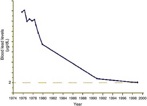
FIGURE 4-3 Blood lead concentrations in the U.S. population from 1976 to 1999. SOURCE: Adapted from CDC 2002.
conventional vehicles, use current technology, and are no more limited in range than current vehicles.
Recently, a much greater use of diesel engines in passenger cars has also been promoted in part as a way to get better fuel economy. Diesel engines have been greatly improved in recent years in noise and smoke production and in cold-starting ability. However, they continue to produce higher NOx and PM emissions than gasoline engines. Great efforts are now under way to devise emission controls to treat these emissions and meet Tier II emission standards.
Beyond the lead phase-out, several states preceded the federal government in regulating motor-vehicle fuels. In the early 1970s, California imposed limits on the Reid vapor pressure (RVP,15 a measure of volatility) of gasoline sold in some parts of the state. RVP affects evaporative emissions of gasoline from vehicles as well as from storage tanks and distribution facilities. California was also the first state to impose limits on the sulfur content of gasoline.
In the years preceding adoption of the 1990 CAA Amendments, increased action by states was focused on the need to regulate fuels in addition to motor vehicles. In 1988, Colorado pioneered oxygenate requirements for gasoline—specifying a minimum oxygen content of 1.5% by weight during the winter—to reduce CO emissions. Several other western states soon followed suit.
In 1989, first the northern states and then the federal government took another step in fuel property regulation, imposing RVP limits for gasoline. At the time, RVP limits, as compared with other various mobile- and stationary-source controls, were judged to be by far the most cost-effective means available for reducing VOCs and, in turn, O3 which had become an important issue because of the pervasive violations of the O3 NAAQS that occurred during the summer of 1988 (OTA 1989). Average RVP levels had steadily risen during the 1980s, in part because of the use of light hydrocarbons to replace tetraethyl lead as octane enhancers (see Box 4-4).
The 1988 California Clean Air Act charged the Air Resources Board with attending to both vehicles and their fuels in pursuit of the maximum possible emission reductions of VOCs and NOx. The Atlantic Richfield Company (ARCO) introduced the first reformulated gasoline (RFG), known as EC-1, in Southern California. EC-1 contained reduced amounts of olefins, aromatics, lead, and sulfur as compared to regular unleaded gasoline; had a lower RVP; and had methyl tert-butyl ether (MTBE) added to raise the oxygen content.
In 1989, a major collaborative program between the automobile manufacturers and the oil industry, known as the Auto/Oil Air Quality Improvement Research Program (AQIRP), tested a variety of fuel and engine combinations designed to reduce emissions (Auto/Oil AQIRP 1993, 1997).
With these precedents, fuel regulations became a significant element of the motor-vehicle emission-control provisions (Title II) of the 1990 CAA Amendments. They mandated the use of RFG during the summer in nine major metropolitan areas with a severe or extreme O3 nonattainment status and allowed additional areas to opt into the RFG program. Winter oxygenated gasoline requirements (oxygen content 2.7% by weight) were mandated for about 40 CO nonattainment areas. The 1990 CAA Amendments also established a nonattainment area fleet program and a California pilot program to encourage the development and use of clean-fueled vehicles. As described in Chapter 2, the RFG program was also intended to reduce emissions of benzene, one of the principal mobile-source air toxics.
The federal RFG program described in Table 4-5 includes both performance requirements, specified in terms of emission reductions, and content
TABLE 4-5 Part 1: California and Federal Reformulated Gasoline Programsa
|
California RFG Program, Phase 1 (1992–1996) |
Federal RFG Program, Phase I (1995–1999) |
|
|
• Effective January 1, 1992. • Set gasoline RVP limit at 7.8 psi. • Required detergent additives and no lead in gasoline. • No explicit oxygen requirement for summer gas. |
• Mandated in 42 U.S.C. 7545 as a result of language in Section 211(k) of the CAA Amendments of 1990. • Effective beginning January 1, 1995, in the 9 metro ozone-nonattainment areas with population of 250,000 or greater classified as “extreme” or “severe” as of November 15, 1990: • Los Angeles (South Coast Air Basin) • San Diego • Baltimore/Washington • Hartford-New Haven-Waterbury, CT • New York/New Jersey/SW Connecticut • Philadelphia/Wilmington/Trenton • Chicago/NW Indiana • Milwaukee/Racine, WI • Houston/Galveston/Brazoria, TX (Sacramento, CA was later added) • Specified content criteria for gasolines to be sold in these areas primarily during the summer ozone season: oxygen minimum of 2.0% by wt; benzene maximum of 1.0% by vol; aromatics maximum of 25.0% by |
|
|
California RFG Program, Phase 2 (1996–) |
||
|
• Effective with beginning of 1996 ozone season. • Set flat limits for the following properties: |
||
|
• RVP: |
7.0 psi (gauge) |
|
|
• Sulfur: |
40 ppm (vol) |
|
|
• Oxygen: |
0–2.7% (wt) |
|
|
• Olefins: |
6.0% (vol) |
|
|
• Aromatics: |
25% (vol) |
|
|
• Benzene: |
1.0% (vol) |
|
|
• Temperature at which 50% of fuel is distilled/vaporized (T 50 ): 210°F. • Temperature at which 90% of fuel is distilled/vaporized (T 90 ): 300°F. |
||
|
• Meets federal Phase II RFG specification and performance requirements (see Table 4-5 Part 2) except that oxygenate content requirement may be waived if a refiner demonstrates, through emissions test results for 20 vehicles in four technology classes, that a fuel’s exhaust-emissions performance targets can be achieved without it. • Properties may be measured according to an average limits provision, as long as the flat limits are met on average over a specified period of time. • RFG performance relative to that of a specified base fuel for exhaust emissions only is calculated with the Predictive Model, which California developed using approximately the same data base that EPA used in developing the Complex Model. |
vol; must contain detergent additive; must exclude heavy metals. • Per-gallon performance requirements: 15.0% reduction in toxics; at least 15.6% northern states; 35.1% southern states; reduction in VOC relative to specified baseline gasoline, as computed by Complex Model (Simple Model valid until January 1, 1998). • Average performance requirements (across all RFGs from a refiner): at least 16.5% reduction in toxics; at least 17.1% northern states, 36.6% southern states; reduction in VOCs as computed by Complex Model (Simple Model valid until January 1, 1998). • RVP limits based on 40 CFR 80.28 standards, which cover all gasolines sold. Other areas may opt into program irrespective of ozone attainment status and may opt out if alternative means of attaining (and maintaining) ambient ozone standards are demonstrated. |
|
aUnless otherwise stated, standards for the first phase of both programs carry forward to the second phase. SOURCE: NRC 1999b. |
|
TABLE 4-5 Part 2: Future Reformulated Gasoline Program
|
Federal RFG Program, Phase II (2000–) |
|
• Effective January 1, 2000. • Revises per-gallon performance criteria for gasolines to be sold in covered and optin areas during the ozone season: at least 20% reduction in toxics; at least 25.9% (northern states) and 27.5% (southern states) reduction in VOCs; and at least 5.5% reduction in NOx (which was not previously controlled) for VOC-controlled areas; relative to specified baseline gasoline, as computed by the Complex Model. • Similarly, if a refiner opts to meet performance criteria on a pooled average (rather than per-gallon) basis as described in 40 CFR 80.67, targets are at least 21.5% reduction in toxics; at least 27.4% (northern states) and 29.0% (southern states) reduction in VOCs (but 23.4% and 25.0%, respectively, for any individual gallon sampled); and at least 6.8% reduction in NOx for VOC-controlled areas; all relative to specified average baseline gasoline, as computed by the Complex Model. • For areas not designated VOC-controlled, the pooled average NOx reduction standard for RFGs is 1.5%. • Per-gallon oxygen minimum requirement relaxes to 1.5% by wt as long as an average oxygen content across all RFGs produced by a refiner for a given area is 2.1% or higher. • Per-gallon benzene maximum requirement relaxes to 1.3% by wt, as long as an average benzene content across all RFGs produced by a refiner for a given area is 0.95% or lower. |
|
SOURCE: NRC 1999b. |
requirements by weight, including a requirement that the fuel contain 2% oxygen (NRC 1999b). The RFG program provides two compliance options to refineries. One is a per-gallon performance requirement ensuring that all fuel sold in program areas meets the standards. The other is a nominally more stringent performance requirement to be met on average across all of the RFG produced by a refinery. To determine whether a specific fuel complies with the performance standards, EPA developed two regression models from laboratory tests of vehicles operated on fuels with a wide range of compositions and properties. These models, known as the simple and complex models, estimate exhaust and evaporative emissions based on fuel properties such as RVP, oxygen content, sulfur content, and the fuel’s distillation curve. Although these models provide a straightforward regulatory framework for refiners and air quality managers to determine whether a given fuel blend meets the specifications required for the RFG program, the output of these models might not accurately reflect the actual performance of the fuels when used with the fleet of cars in operation (NRC 1999b).
Phase II of the federal RFG program took effect in January 2000. It tightens the performance standards, as shown in Table 4-5, allowing refineries to choose between per-gallon or on-average compliance options. Currently, the RFG program is required in 10 metropolitan areas: Los Angeles, San Diego, Baltimore-Washington, Hartford, New York, Philadelphia, Chicago, Milwaukee, and Houston, as specified in the 1990 CAA Amendments, and Sacramento, which was added when it was reclassified as a severe nonattainment area in 1995. Thirteen metropolitan areas or states are voluntarily participating. In addition, Phoenix has its own, more stringent RFG program (EPA 2002j).
In addition to the federal RFG program requirements, Table 4-5 shows the California RFG program’s distinct requirements. That program was implemented on an accelerated schedule: Phase 1 of the California program started in 1992 and Phase 2 in 1996. Phase 3, which includes a ban on the use of MTBE, was originally scheduled to start on December 31, 2002, but has been postponed until December 31, 2003 (CARB 2003a), because of delays in removing the CAA oxygen requirement for RFG.
Oxygen-content requirements for RFG (2% by weight) and oxygenated fuels (2.7% by weight) mandated by the 1990 CAA Amendments have been controversial. Although the motivation for including them in the 1990 Amendments was ostensibly to aid in the reduction of emissions, they were also motivated strongly by a desire on the part of the sponsors from farm states to increase the use of ethanol in the fuel supply for purposes of farm policy and for decreasing reliance on foreign sources of oil (EPA 1999f). Ethanol and MTBE are the two additives most widely used to meet the oxygen content requirement, MTBE being used most heavily outside the
Midwest. The addition of ethanol to gasoline can increase its RVP, in turn, increasing evaporative emissions from vehicles as well as from the fuel storage and distribution system. The net impact on air quality of adding ethanol to fuel is small but under some circumstances might be negative. MTBE does not increase RVP, but leaking gasoline storage systems have contaminated groundwater and raised health concerns (NSTC 1997). An NRC (1999b) report concluded that although adding oxygenates to gasoline reduces CO in vehicle exhaust, as well as the evaporative and tailpipe emissions of some air toxics, it has little effect on exhaust emissions of VOCs and may increase exhaust emissions of NOx. Because of concerns about the oxygen additives, CARB requested a waiver from EPA from the oxygen content requirements of the RFG program, arguing that the requirement impeded its efforts to reduce NOx emissions. A blue ribbon panel convened by EPA to review the matter in 1999 recommended a substantial reduction in the use of MTBE and the removal of the RFG oxygen content requirements (EPA 1999f). Although EPA denied California’s request, it has supported changes to the program. Congress is considering amendments to energy legislation that would ban MTBE and replace the oxygen requirement with a renewable fuels requirement that would likely substantially increase ethanol use.
For CO emissions, the benefits of oxygenated fuel use are most pronounced in older vehicles. New vehicles with properly functioning closed-loop control systems show relatively little benefit.16 Thus, the effectiveness of the oxyfuels program has diminished as the vehicle fleet has turned over. The CAA Amendments of 1990 do not have a sunset provision for the oxygenated fuels requirement, but in effect this requirement has been diminishing as a large portion of locales with high ambient CO concentrations have attained or are close to attainment of the CO NAAQS.
In addition to the emission standards promulgated in the new Tier 2 emission standards for passenger vehicles, including SUVs, minivans, and other LDTs, EPA is imposing new restrictions on sulfur in gasoline, primarily to prevent sulfur-poisoning of catalytic converters (65 Fed. Reg. 6698 [2000]). In 2004, corporate average sulfur concentrations of 120 ppm with a cap of 300 ppm will be required. By 2006, the corporate average limit will be reduced to 30 ppm and the cap to 80 ppm. The regulations will be phased in more slowly for gasoline produced for sale in the western United States and for small refiners. They also allow refiners to generate credits for
reductions achieved ahead of schedule; refiners may then apply these credits toward meeting their regulatory requirements or transfer them to other refiners or importers.
Like the Tier 2 LDV standards, EPA’s new emission standards for heavy-duty diesel engines, published in January 2001, are also accompanied by tightened limits on fuel sulfur content to prevent catalyst damage (66 Fed. Reg. 5002 [2001]). Starting in 2006, the new sulfur limit for most diesel fuel will be 15 ppm. Through 2009, up to 20% of diesel may still be produced with a sulfur content of up to 500 ppm, but it may only be sold for use in pre-2007 engines. As with the gasoline rule, small refineries have a slower phase-in schedule. Refineries producing diesel fuel and gasoline for sale in the western states may stagger their compliance schedules for the two fuels. The regulation also includes an averaging, banking, and trading component. Here, refineries can generate credits on the amount of 15-ppm sulfur diesel fuel that exceeds their required 80% production. These credits may be averaged with another facility owned by that refinery, banked, or sold to another refinery.
BEHAVIORAL AND SOCIETAL STRATEGIES TO REDUCE MOBILE-SOURCE EMISSIONS
Although individual vehicle emissions have been reduced substantially over the past 30 years, those improvements have been offset at least partially by continued increases in vehicle miles traveled (VMT). Thus, controls on vehicle activity and transportation represent a potentially important avenue for reducing emissions from mobile sources.
Regulation of Motorists’ Vehicle Use
Under the CAA Amendments of 1970, EPA required the states to develop transportation control plans (TCPs) for their air pollution control areas (normally, metropolitan regions). The TCPs were to be incorporated into the overall SIPs for attaining and maintaining compliance with the NAAQS. Because the 1970 CAA Amendments required attainment of the standards by 1975, it appeared that stringent transportation controls would be required in many areas; for example, parking supply restrictions, high taxes or surcharges on parking, and downtown access restrictions. These policies proved highly unpopular, however, and most states refused to submit TCPs (Howitt and Altshuler 1999).
In 1973, EPA promulgated federal TCPs for 19 major metropolitan areas that included the types of policies that the states had chosen not to impose on their own authority (Altshuler et al. 1979; Suhrbier and Deakin 1988). Congress then restricted EPA’s authority to require price disincen-
tives (such as road-use tolls and parking surcharges) or to restrict parking at all, and EPA effectively abandoned efforts to enforce the federal TCPs (Altshuler et al. 1979; Howitt and Altshuler 1999).
The 1977 CAA Amendments did not mandate restrictions on personal travel, although they permitted states to adopt restrictions if they wished. They also authorized the federal government to withhold most federal highway funds from any state failing to submit an acceptable SIP to EPA (Howitt and Altshuler 1999). Although the states did submit their SIPs, very few proposed or implemented controls on personal travel (Horowitz 1978; Deakin 1978; National Commission on Air Quality 1981; Yuhnke 1991).
The CAA 1990 Amendments again left the decision of whether to adopt transportation control measures to state and local officials, with one major exception: mandated employer trip reduction programs (the employee commute options [ECO] requirement) in the 10 most severely polluted nonattainment areas. Some of the 10 affected areas initially proceeded with EPA’s ECO program, requiring employers to reduce the amount of automobile commuting to their work sites. Beginning in 1994, EPA found it difficult to defend the ECO program against growing resistance from business groups because few emission-reduction benefits were expected from the program. Congress made the program voluntary in December 1995 (Public Law 104-70).
Outside the United States, there have been a number of efforts to try to address motorist behavior. These include strict restrictions in Singapore (Chia and Phang 2001), alternate day vehicle restrictions in a number of cities, and recent efforts to impose a user fee for drivers into central London. Although these programs may provide some useful insights, some have been implemented in very different governmental circumstances (for example, the authoritarian practices of the Singapore government). Also, others have taken place in the context of broader government policies that have imposed a much higher cost of fuel than is politically realistic in the United States. Still others, such as the London experiment, are not substantially different from programs already in place in the United States. For example, the cost of crossing the Hudson River into New York City is already nearly as high as the new charge imposed in London.
Regulatory and other efforts under the CAA to reduce motor vehicle use have proved to be politically infeasible. On the other hand, some efforts to promote voluntary reductions in vehicle use, such as ride-sharing programs, enhancement of existing transit service, compressed work weeks, and telecommuting, have won political acceptance. However, such programs generally have little potential to affect overall use of motor vehicles; each is expected to yield about 1–3% reductions in VMT (Apogee Research 1994; Howitt and Altshuler 1999).
Controls on Transportation Infrastructure Planning and Investment
Another class of strategies that can be undertaken to reduce motor-vehicle emissions focuses on optimizing urban and regional transportation patterns and practices. Such strategies require careful integration of urban and regional plans for land use, transportation infrastructure, housing, and economic development. Because they are implemented on decadal time scales, their successful implementation requires a continuing commitment on the part of local and regional managers and politicians to long-term air quality improvement.
Within the general theme of transportation planning and AQM, highway capacity has become a highly contentious and complex issue. Because free-flowing traffic at moderate speeds produces less pollution per vehicle mile than highly congested traffic produces, construction of additional highway lanes and access roads would seem to improve air quality. However, highway expansion in a metropolitan area can encourage urban sprawl and low-density development (TRB 1995). Low-density development, which, in turn, increases the number and length of vehicle trips, decreases vehicle occupancy rates, and diminishes the practicality of pedestrian and transit trip making. Similarly, road building to alleviate congestion in densely developed corridors may induce additional travel, because a great deal of latent travel demand in such areas invariably has been suppressed by the existing congestion. The end result can be an increase in automobile travel and increased mobile-source emissions.17
Linking Highway Capacity Expansion to Air Quality through the National Environmental Policy Act
In its initial forms, the SIP process lacked a formal procedure to ensure that automobile usage and VMT projections used by air quality planners in NAAQS attainment demonstration were consistent with regional plans for highway and road construction. Before the 1990 CAA Amendments, neither federal law nor the practices of metropolitan transportation planning linked air quality management with urban transportation investment policy. The National Environmental Policy Act (NEPA) of 1969 had attempted to address this problem by mandating that federally funded projects be broadly analyzed for their impacts on the environment. However, NEPA only required that environmental impacts be considered in evaluating projects; it did not provide substantive guidelines for permitting projects to proceed to construction, nor did it require consistency with the projections used in
SIPs. In addition, NEPA’s project-by-project focus did not generally consider the cumulative environmental effects of multiple projects.
Further efforts to create links between air quality regulation and regional transportation planning and investment encountered significant institutional problems and resistance. Section 109(j) of the Federal-Aid Highway Act of 1970 required the secretary of transportation, in consultation with the EPA administrator, to issue regulations for the purpose of ensuring that federally assisted highway projects were consistent with the air quality plans for each pollution control area. However, the regulations were vague on the question of how consistency should be determined, and they had state transportation officials, rather than environmental regulators, making the consistency determinations. In most areas, EPA regional offices made little effort to activate Section 109(j). The 1977 CAA Amendments contained stronger language but were only marginally more effective (Howitt and Altshuler 1999).
The Conformity Regulations
The CAA Amendments of 1990 and the Intermodal Surface Transportation Efficiency Act (ISTEA) of 1991 required much tighter integration of (or conformity between) clean air and transportation planning (Howitt and Moore 1999a). The conformity regulations most directly affect metropolitan planning organizations (MPOs), the public agencies that conduct transportation planning under federal transportation law (ISTEA from 1991 to 1997 and TEA-21 [Transportation Equity Act for the 21st Century] since then). Other agencies and stakeholders also play a role. A significant aspect of the conformity regulation is the incentive given to both air quality and transportation planners to maintain conformity. The penalty for non-conformity is a transportation funding cutoff. For some metropolitan areas, that can mean the loss of more than $100 million per year.
At the core of the conformity requirement is an EPA-mandated analytical procedure and regulatory test to ensure that transportation-related emissions in a nonattainment area stay within the limits used in the area’s SIP. As described by Howitt and Moore (1999a), the process involves use of a computer simulation to make a 20-year forecast of emissions from the transportation system. The forecast takes into account changes in demographics, land use, economic development, and transportation infrastructure and services. The forecasted emission concentrations are compared with the maximum emissions permissible in certain milestone years under the state’s SIP. If those concentrations exceed permissible levels in the SIP, an MPO must change its transportation plans and programs so that forecasted emissions would be within the emission budget constraints. Alternatively, the state must amend its SIP to reduce transportation-related
emissions through additional mobile-source control measures or reduce emissions from stationary sources, such as industrial facilities or smaller area sources. In addition, an MPO must demonstrate timely implementation of transportation control measures in SIPs and fulfill the ISTEA “fiscal-constraint” requirement for transportation plans and programs by showing that it is likely to have sufficient financial resources to carry them out.
If an MPO cannot satisfy the conformity requirements within specified time periods, then penalties are imposed during a conformity “lapse” or “freeze.” During this time, the MPO may not begin most new transportation projects, and the use of federal transportation funds is restricted. Conformity lapses or freezes can also result from certain shortcomings in a SIP, which may or may not involve transportation-related issues (Howitt and Moore 1999a).
To date, the most widespread effects of conformity have been procedural and cultural. Before the conformity regulations of the 1990 CAA Amendments, transportation planning and air quality regulation were effectively separate spheres of government activity, even within a given state. Conformity appears to have fostered greater interaction; as a result, it is likely that transportation and environmental agencies have gained more knowledge about and a greater appreciation for one another’s missions, responsibilities, and procedures. Most transportation officials also seem to accept the legitimacy and high priority of environmental values in transportation decision-making (Howitt and Altshuler 1999).
Thus far, the conformity requirement has had the largest impact on NAAQS nonattainment areas experiencing rapid growth and, therefore, substantial economic and political pressure to expand transportation infrastructure. Atlanta, Charlotte, and Houston, for example, have had federal transportation funding interrupted because of conformity problems. As further emission reductions are required in the years ahead, nonattainment areas that are rapidly growing are likely to experience conformity as an increasingly salient constraint. It is uncertain how the conflicts between transportation and air quality goals in such areas will be resolved and whether the federal government will remain firm in enforcing the regulation.
The conformity requirement has had less impact on transportation planning in older, more slowly growing metropolitan areas. These areas have more mature highway networks and well-established transit systems, and most of their transportation projects, involving highway and transit reconstruction and modest expansions, are neutral or positive in terms of air quality. In addition, these areas often have more serious air pollution problems and thus more time to come into compliance with the CAA (see Table 3-1 in Chapter 3). Therefore, conformity has not required these
areas to make major adaptations. However, these regions have not yet met their stiffest challenges, because they still must demonstrate future reductions in transportation-related emissions (Howitt and Moore 1999b).
CRITICAL DISCUSSION OF MOBILE-SOURCE EMISSION-CONTROL PROGRAMS
The CAA has led to substantial successes in some aspects of its mobile-source programs. The emissions standards for individual LDVs and HDVs have promoted a host of new technologies, which have resulted in or are expected to result in emissions that are substantially lower than they were in 1970. These emission standards also resulted in eliminating the largest source of lead in the environment through the control of lead in fuels. Despite increasing travel, which has offset some of the gains, the number of communities having air that is not in attainment of the NAAQS for lead or CO (pollutants that are primarily from mobile sources) has dropped dramatically. As described in a recent NRC (2003b) report, that drop has resulted in substantial reductions in overall population exposures to high concentrations of ambient CO.
Mobile-source emission-control programs have also experienced and continue to experience challenges, including the persistence of high-emitting gasoline vehicles and older diesel vehicles, the relative lack of regulation of nonroad engine emissions, the contributions of mobile sources to HAP emissions (see discussion of HAPs in Chapter 5), the use of fuel policy to pursue other non-air-quality-related interests (for example, farm policy and reducing dependence on foreign oil), and the inability of AQM to affect individual travel behavior substantially.
The following section reviews and summarizes some of the lessons learned and the challenges ahead.
Promotion of New Technologies Using Vehicle Emission Standards
The history of vehicle emission controls is one of long-term success, albeit success that came more slowly than policy-makers originally intended. Delays were due in part to opposition from the automotive industry facing the challenge of producing the required technologies in a cost-effective manner. Nonetheless, substantial improvements in technology have occurred: more efficient combustion resulting in fewer partially combusted hydrocarbons; emission-control systems with longer effective lifetimes; and the application of many new catalyst and sensor technologies, using increasingly sophisticated computer controls. Actual costs of the improvements have often proved to be less than anticipated (Anderson and Sherwood 2002; Cackette 1998). Lower costs were realized as production
experience was acquired, economies of scale were achieved, and the desire to meet a mass market had fueled substantial competition. Some observers have suggested that such economies are more likely when policies target a relatively small number of large corporations and focus on inducing substantial (but not radical or technologically infeasible) changes in product technology (Howitt and Altshuler 1999).
Even so, the process can be marked by considerable controversy and even litigation. Delays are often unavoidable, and accommodations between legislative purposes and industry interests are a frequent part of the implementation process. Nevertheless, the technology promotion process appears to be able to provide the nation with a significant mitigation of air pollution in a cost-effective manner (Howitt and Altshuler 1999).
High-Emitting Gasoline Vehicles
The emission-control program for mobile sources has been very successful in terms of its ability to reduce emissions from individual LDVs, operated in normal modes. The forecast emission reductions from recently promulgated regulations, if fully effective over the lifetime of an operational vehicle, will provide a further dramatic reduction in mobile-source emissions. However, analyses suggest that historically, a disproportionately large fraction of the mobile emissions come from a relatively small percentage of so-called high-emitting cars. Many of these high emitters are vehicles whose pollution control devices are not operating properly or whose engines are combusting combinations of fuel and lubricating oil. In addition to representing significant sources of VOC, NOx, CO, and air toxics, high-emitting gasoline vehicles might also be significant contributors to ambient concentrations of PM2.5 (Watson et al. 1998). That possibility suggests that attainment of the new NAAQS for PM2.5 will require a much better understanding of the effect of engine operation and deterioration on the emissions of fine particles from gasoline vehicles.
The continued presence of high emitters, which were first described by Wayne and Horie (1983) and which continue to be observed in the contemporary vehicle fleet (NRC 2001c and references therein), will reduce the emission reductions that are forecast for programs to be implemented in the latter half of this decade. To date, the nation’s AQM system has not come up with an effective and politically acceptable means to address this problem. One mechanism, which appears to have been at least partially successful, has been to require increasingly durable, warranted emission-control systems, resulting in substantially more robust emission-control systems. New vehicles are currently certified to 100,000 mile standards and major emissions control equipment, such as the catalyst and on-board computer, are warranted for 80,000 miles. Other mechanisms, such as inspection and
maintenance and remote sensing, have been either politically controversial, technically ineffective, or both. A further opportunity, as yet unrealized, might lie in the improvement and monitoring of on-board diagnostic devices that immediately notify drivers of problems and in the long run provide officials and mechanics with accurate information on the performance of emission-control equipment.
Reducing Emissions from Older and Nonroad Diesel Engines
Although there has been and probably will be substantial progress in reducing the emissions from new on-road diesel vehicles, three substantial challenges remain. First, the long life of diesel vehicles and the pattern in which older vehicles are used for shorter-haul routes in urban centers result in a large and continuing source of PM and NOx diesel emissions in urban settings with dense populations. Recent efforts by the states and EPA to promote buy-back, replacement, and retrofit programs have begun to address this issue, but these efforts have been modest. Second, the recent enforcement experience with on-road emissions being higher than those certified for the engines and the difficulty of inspection and maintenance for heavy-duty engines will require continued attention. Finally, as on-road LDV emissions continue to decline, emissions from various nonroad sources and on-road diesel vehicles will become increasingly important. Recent regulatory efforts by EPA (as detailed above) have begun to address this last issue. Although these recent efforts have begun to address the issue of in-use heavy-duty vehicle emissions, there is not yet a systematic, nationwide approach to the problem. Specific recommendations for addressing this problem are advanced in Chapter 7.
Regulating the Content of Gasoline and Diesel Fuels
The past 15 years have seen a substantial increase in CAA programs regulating the composition of fuel. In some instances, these programs have been directly responsible for substantial decreases in exposure to important air pollutants—most notably, lead—and for a substantial reduction in benzene emissions and exposure with the advent of RFG. The elimination of sulfur is also likely to facilitate a new generation of gasoline and diesel control technologies, as occurred with the removal of lead in the 1980s. This potential for further technological innovation, however, depends on the successful implementation of the sulfur-reduction regulations on the time scale envisioned in the regulations.
The success of these new fuels in reducing key precursors for O3 is less clear. Congressional requirements for oxygen in RFG that resulted in increased use of ethanol may have resulted in increasing evaporative emis-
sions and, in some instances, a worsening of O3 conditions (NRC 1999b). As indicated above, such actions were taken not only for air quality reasons but also for other reasons (for example, farm policy and energy security). The challenge of reducing O3 precursors is made larger by the limitations of the current technical tools available for predicting motor vehicle emissions as a function of the fuel blend (for example, the Simple and Complex models used for RFG). For MTBE, the oxygen requirements also resulted in increasing the risk of groundwater and surface-water contamination (EPA 1999f).
One advantage of such programs has been to reduce emissions in older, less well-controlled vehicles. However, many of these older LDVs have now been replaced, but there is no provision for reviewing and, if appropriate, removing specific fuel requirements as the older LDVs are replaced. Finally, Tier II fuel requirements have included banking, averaging, and trading provisions to improve the cost-effectiveness of the rules. To date, however, with the exception of the lead phase-out, there has not been adequate experience to evaluate these programs and to determine their effectiveness. Such evaluation will be especially important as EPA implements the new sulfur-reduction requirements, and extends them to nonroad diesel fuel.
Controls on Motorists’ Behaviors
In contrast to the success of new motor vehicle standards, efforts to regulate citizen’s personal travel behavior through restrictions or economic disincentives have typically provoked controversy and, in the end, have proved to be politically infeasible. Even where some effort has been made, the estimated pollution reductions have been modest. After 30 years of efforts to affect individual driving behavior, all involved—Congress, EPA, and state and local agencies—have opted to emphasize voluntary versions of such efforts (Howitt and Altshuler 1999).
Conformity
In the related area of regulation of infrastructure investments, some modest progress appears to have been made. The 1970 and 1977 CAA Amendments were ineffective in ensuring consistency between state transportation investments and air quality improvement commitments. The 1990 CAA Amendments embodied a more realistic appreciation of how transportation decisions can affect air quality planning and backed the requirement for conformity with the tangible threat of federal fiscal penalties for failure to comply. The invigorated “conformity” requirement appears to have enhanced the attention paid to air quality objectives in metro-
politan transportation planning, although it has not, to date, significantly affected state transportation investment decisions.
Perhaps the most important substantive effect of conformity may be a new way of looking at highway projects in the early stages of the transportation planning process. Proposals for major highway enhancements, which can be “emission budget busters,” may now be less likely to move into the preliminary planning stage, particularly because planners must show that the financial resources needed to carry out the proposals are likely to be available.
Only a few rapidly growing areas have been motivated by conformity requirements to pursue major investments in mass transit, because such investments rarely produce significant air quality benefits. In the areas that already have extensive transit networks, however, the conformity requirements have reinforced the importance of modernization, service enhancements, and occasional extensions (Howitt and Moore 1999b).
The relationship between SIP development and the conformity process can create difficulties for both planning and regulatory purposes for several reasons: assumptions, data, and forecasts. These difficulties occur when the two planning processes are insufficiently interconnected. The federal conformity regulations mandate the use of the most up-to-date transportation-planning assumptions and data available (for example, for travel behavior, population, land use, and economic growth) and the most recent version of the emission forecasting models (that is, EPA’s MOBILE model or California’s EMFAC model). Because conformity analyses must be revised at least every 3 years in nonattainment areas and SIPs might not be updated for much longer periods, the underlying assumptions, data, and models used in the transportation-planning process may vary significantly from those in the air quality plan. The disjunction of modeling inputs and methods, depending on the circumstances, can create differences in estimates of future emissions that may only exist on paper in the planning process or mask real air quality problems. Thus, the disconnection between SIP development and the conformity process undermines the intended usefulness of conformity as a performance test allowing informed judgment of whether state transportation investments are consistent with air pollution reduction commitments in the SIP. Moreover, the planning horizons for air quality regulation and transportation planning may mesh poorly. Under current requirements, transportation plans are required to have a 20-year time horizon, and conformity is done on that basis. An attainment demonstration and associated maintenance plan, however, need only a 10-year time horizon. Transportation plans must therefore often use emission budgets that do not take account of future emission growth in transportation and other sectors (Harrington et al. 2003).
Both the possible disjunction of planning assumptions and forecasts between SIPs and conformity analyses and the poorly meshing time frames
of the two processes can create important questions about regulatory fairness. The procedures of the CAA were designed so that, in setting emission budgets, decision makers would take forecasts of aggregate emissions and then explicitly allocate emission estimates across sectors in ways that created legitimacy and stakeholder commitment to the outcome. If transportation emission forecasts are updated while other sectors’ are not, the validity and perceived fairness of the results can be questioned and stakeholder support for pollution reductions can be undermined.
Some proponents of conformity hoped that linking transportation and land use would encourage broader acceptance of land-use regulations to reduce emissions from mobile sources. However, the impact of conformity on land-use decision-making, which is in the hands of local governments that do not have a direct role in conformity, has been modest (Howitt and Moore 1999a).
SUMMARY
Strengths of the Mobile-Source Emission-Control Program
-
Regulations on LDVs and LDTs have resulted in significant reductions in the emissions per mile traveled. In the case of CO, as shown in a recent NRC study (NRC 2003b), those reductions have resulted in significant reductions in overall population exposure. Further emission reductions are anticipated from the implementation of stricter emission regulations in the coming years.
-
Emission regulations on LDVs and LDTs have promoted the development and application of new cleaner technologies for vehicles—technologies that are now used worldwide. Furthermore, the actual costs of these technologies were likely less than anticipated.
-
Regulations on fuel properties, including content, have also resulted in air quality benefits, most notably is the phase-out of lead in gasoline that made the use of catalytic converters possible and reduced population exposure to lead. RFG resulted as well in reductions in population exposure to benzene. New regulations on sulfur content in fuels promise to further enhance the effectiveness of catalytic controls and reduce emissions of the on-road fleet.
Limitations of the Mobile-Source Emission-Control Program18
-
Gaps remain in the ability to monitor, predict, and regulate in-use vehicle emissions. The existence of high emitters is a major challenge, and
|
18 |
Recommendations are provided in Chapter 7. |
-
I/M programs have been less effective than expected in identifying high emitters and ensuring in-use compliance with emission standards. Other approaches, such as remote sensing and on-board diagnostics, show technical promise, but further testing of those techniques is needed. There is also a concern that remote sensing may be viewed as unacceptably invasive.
-
As emissions from LDVs and LDTs decrease and the focus on attaining the NAAQS for PM2.5 increases, emissions from nonroad engines and heavy-duty onroad vehicles are becoming increasingly important. New emission regulations for these sources are being implemented, but the long lifetime of these engines will slow the rate of penetration of the effects of these regulations into the fleet. Additional efforts in inspection and maintenance and in promoting retrofit and incentive buy-back programs are therefore needed.
-
The inclusion of content-specific requirements in the fuel provisions of the 1990 CAA Amendments (for example, oxygen in the RFG program) can limit flexibility to meet standards in the most cost-effective way for areas required to implement the program. The standards also make it difficult to adjust the program in the face of new challenges (for example, in the case of MTBE contamination of groundwater and surface water) and have a small (sometimes even negative) impact on the control of some air pollutants (as might have been the case with the use of ethanol and potential increases in RVP).
-
Growth in vehicle miles traveled, personal automobile usage, and popularity of fuel-inefficient vehicles (for example, SUVs) has offset a significant portion of the gains obtained from stricter emission standards on individual vehicles. With the exception of the conformity requirements of the 1990 CAA Amendments and subsequent related legislation, air quality managers remain unable to affect these societal and behavioral determinants of mobile-source emissions.


