
6
Measuring the Progress and Assessing the Benefits of AQM
INTRODUCTION
Implementation of the Clean Air Act (CAA) via the procedures and methods described in Chapters 2 through 5 has resulted in significant improvements in air quality in the United States, according to the U.S. Environmental Protection Agency (EPA), and these improvements have had a positive impact upon public health and welfare. EPA estimated that emissions of the six criteria pollutants have decreased by about 30% over the past three decades, despite sizable increases in population, energy use, and gross domestic product (see Figure 1-4 in Chapter 1). The estimated benefits of these reductions are substantial; they include an estimated 100,000 to 300,000 fewer premature deaths per year and 30,000 to 60,000 fewer children each year with IQs below 70 (EPA 1997). In economic terms, these benefits have been estimated to amount to trillions of dollars. In this chapter, the committee discusses how such estimates of the progress and benefits of AQM in the United States are made, the uncertainty of the estimates, and what can be done to reduce the uncertainty.
MONITORING POLLUTANT EMISSIONS
Direct Measurement
The most direct way to confirm that specific emission-control technologies are working effectively is to measure the rate at which pollutants are released from relevant sources. However, with a few exceptions, pollutant
emissions are not routinely monitored in the United States. One notable exception is the congressional requirement for continuous emissions monitoring (CEM) of sulfur dioxide (SO2), nitrogen oxides (NOx), and particulate matter (PM) from any source regulated under the acid rain provisions of the 1990 Amendments to CAA. As discussed in Chapter 5, the inclusion of such monitoring is viewed as being essential to ensuring the success of the cap-and-trade mechanism incorporated into the legislation. Moreover, the application of CEM has provided direct evidence of substantial reductions in SO2 emissions from utilities since the implementation of the acid rain controls (see Figure 5-1 in Chapter 5). Inspection and maintenance (I/M) programs for motor vehicles, which were mandated in the CAA, could serve, in principle, as a check on the effectiveness of mobile-source emission controls. However, as discussed in Chapter 4, the effectiveness of I/M programs has been limited because of shortcomings in program design and effectiveness, and public resistance to such programs in some areas of the country.
There are a number of reasons why emissions are not routinely monitored. There are myriad stationary and area sources that contribute to pollution, and technologies are not available to monitor their emissions routinely and reliably. Given the resources and measurement technologies available to the AQM system, a program that attempted to monitor emissions comprehensively through direct measurement would be unrealistically expensive and complex. In addition, efforts by the government to monitor certain types of emissions on a continuous basis (for example, mobile emissions) might be viewed by some as an unacceptable invasion of privacy. On the other hand, the application of new technologies and creative measurement strategies could help to make the task more tractable and less invasive. For example, a number of emerging technologies and methods could be deployed to augment I/M for mobile emissions. Remote sensors have been used to identify high-emitting vehicles without inconveniencing motorists or interfering with traffic (Stedman et al. 1997; Bishop et al. 2000); on-board diagnostic systems are being developed to automatically monitor and document problems that lead to increased emissions from individual motor vehicles; and standard air quality monitors could be deployed inside tunnels and along roadways to help characterize in-use emissions from fleets of vehicles (Kean et al. 2001). As discussed in Chapter 5, CEM technologies are very valuable in tracking stationary-source emissions and could be used more widely, but the development of a broader range of CEM systems has been slow.
Using Ambient Concentrations to Confirm Emission Trends
EPA estimates that nationwide emissions of volatile organic compounds (VOCs), SO2, PM, carbon monoxide (CO), and lead (Pb) have decreased
substantially since the early 1980s; the decrease in NOx emissions is estimated to be more modest (see Table 6-1, part A). These emission decreases can be reasonably ascribed to the promulgation of emission controls related to the nation’s implementation of the CAA requirements. Because the importance of NOx for ozone (O3) control was not recognized until the late 1980s or early 1990s, the slower pace of NOx emission decreases, compared with other pollutants, is probably due to the later implementation of NOx controls.
The decline of pollutant emissions during a period of substantial growth in population, energy consumption, and gross domestic product in the United States is cited by EPA and others as evidence of the substantial progress of the AQM system. However, the trends listed in Table 6-1, part A, have been developed from inherently uncertain emission inventories (see Chapter 3), so significant uncertainties must also be attached to the emission trends portrayed in EPA’s reports. Because of such uncertainties, a technically robust AQM system should have mechanisms in place that could
TABLE 6-1 Summary of EPA’s Trends in Estimated Nationwide Pollutant Emissions and Average Measured Concentrations
|
Pollutant |
1983–2002 |
1993–2002 |
|
A. Changes in Estimated Pollutant Emissions, %a |
||
|
NOx |
–15 |
–12 |
|
VOC |
–40 |
–25 |
|
SO2 |
–33 |
–31 |
|
PM10b |
–34c |
–22 |
|
PM2.5b |
No trend data available |
–17 |
|
CO |
–41 |
–21 |
|
Pb |
–93 |
–5 |
|
B. Changes in Measured Ambient Pollutant Concentrations, % |
||
|
NO2d |
–21 |
–11 |
|
O3 1-hr |
–22 |
–2 |
|
O3 8-hr |
–14 |
+4 |
|
SO2 |
–54 |
–39 |
|
PM10 |
No trend data available |
–13 |
|
PM2.5 |
No trend data available |
–8e |
|
CO |
–65 |
–42 |
|
Pb |
–94 |
–57 |
|
aNegative numbers indicate reductions in emissions and improvements in air quality. bIncludes only directly emitted particles. cBased on percentage change from 1985. dThe trends in NO2 should be viewed cautiously because of potential artifacts from the instrumentation. Also, because NO is readily converted to NO2 in the atmosphere, ambient monitoring data are reported as NO2. eBased on percentage change from 1999. SOURCE: Adapted from EPA 2003. |
||
independently establish the validity and accuracy of emission trends derived from emission inventories. Given the current inability to monitor all emissions comprehensively, trends cannot be verified directly. However, in principle, verification can be done indirectly by using long-term measurements of primary pollutant concentrations in the ambient air. The underlying assumption of this approach is that, all things being equal, there should be an approximate 1:1 relationship between a change in the total emissions of a primary pollutant (for example, CO and SO2) and a change in the pollutant’s average atmospheric concentration. Although this approach is straightforward in concept, it can be difficult to implement without an appropriately designed network of pollutant monitors.
Since the 1980s, the United States has had an extensive air quality monitoring network that routinely measures the concentrations of selected air pollutants in some locations. (The objectives and features of this network are discussed in some detail in the next section.) Trends in the concentrations of relevant air pollutants derived by EPA from data obtained from this network are listed in Table 6-1, part B. Initial inspection of these trends indicates qualitative consistency with the estimated pollutant emission trends discussed above—that is, the trends of both emissions and concentrations are downward. However, a more detailed quantitative comparison of the trends indicates significant inconsistencies. As illustrated in Figure 6-1, the downward trends in the average pollutant concentrations tend to be significantly greater than those of the emissions.1 That result could be interpreted to mean that pollutant emissions have decreased more than estimated from emission inventories. However, there are other viable explanations. Significant uncertainties can exist in the concentration trends derived from the nation’s air quality monitoring network (see later discussion on trends analysis). More important, the nation’s air quality monitoring network was not designed to track nationwide emission trends or evaluate emission inventories; instead, it was largely designed to monitor urban pollution levels and compliance with National Ambient Air Quality Standards (NAAQS). As a result, most of the sites in the air quality monitoring network are urban; thus, the trends derived from them are more representative of urban pollution trends than national trends. Because many emission controls on stationary sources between 1970 and 1990 were aimed at urban emissions, urban areas might be expected to have larger decreases in pollutant concentrations than those seen overall. In any event, it would appear that air quality monitoring data provide qualitative but not quantitative confirmation that pollutant emission trends are downward (especially in urban areas) in the United States.
|
1 |
PM10 is an exception; however, note that the emissions change plotted in Figure 6-1 for PM10 is based on the estimated change from 1985 to 2002 and not 1983 to 2002. |
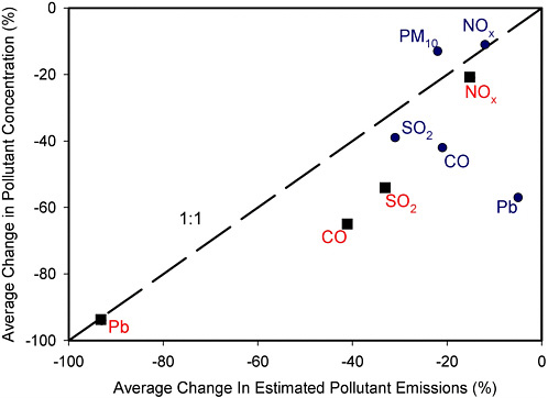
FIGURE 6-1 Scatterplot of estimated trends in pollutant emissions derived from emission inventories and changes in average pollutant concentrations derived from air quality monitoring networks. The squares indicate the trends for the period 1983–2002 (except for PM10 emissions, which are for the trend period 1985–2002) and the circles for 1993–2002. SOURCE: Data from EPA 2003.
MONITORING AIR QUALITY
The 1977 Amendments of the CAA state that
the Administrator shall promulgate regulations establishing an air quality monitoring system throughout the United States which (1) utilizes uniform air quality monitoring criteria and methodology and measures such air quality according to a uniform air quality index, (2) provides for air quaity monitoring stations in major urban areas and other appropriate areas throughout the United States to provide monitoring such as will supplement (but not duplicate) air quality monitoring carried out by the States required under any applicable implementation plan, (3) provides for daily analysis and reporting of air quality based upon such uniform air quality index, and (4) provides for record keeping with respect to such monitoring data and for periodic analysis and reporting to the general public by the Administrator with respect to air quality based upon such data.
In response to this and subsequent congressional mandates, EPA has overseen the development and operation of several national monitoring networks. These networks generally fall into one of two categories: ambient air quality monitoring networks that measure the atmospheric concentrations of pollutants at various locations, and deposition networks that measure the rate at which pollutants are deposited on the earth’s surface. Collectively, these networks provide the best and most detailed (although by no means comprehensive) data available today for assessing the progress of the AQM system.
Because air quality and atmospheric deposition can exhibit large daily, seasonal, and interannual variations independent of any changes in pollutant emission rates, long-term monitoring is needed to detect and interpret air quality trends and thereby determine the effectiveness of regulations. The requirement for complete, precise, and accurate long-term monitoring of air quality presents significant technical challenges that require substantial investments in financial and human resources. In the United States, more than $200 million is spent annually to support air monitoring (EPA 2002p). In addition to providing an essential performance measure of the effectiveness of air quality regulations, air quality monitoring networks provide critically important information to scientists attempting to advance the understanding of the causes and remedies of air pollution. Thus, these networks represent a valuable and significant national resource.
The major federally supported monitoring networks for atmospheric composition and deposition operating in the United States are summarized below and in Table 6-2. An example of the spatial distribution of one of these networks (used to monitor O3) is presented in Figure 6-2.
Atmospheric Composition Monitoring Networks
National, State, and Local Air Monitoring Stations
The CAA requires every state to establish a network of air monitoring stations for the criteria air pollutants. These networks are called the state and local air monitoring stations (SLAMS). SLAMS currently consist of approximately 4,000 monitoring stations whose size and distribution is largely determined by the needs of state and local air pollution control agencies to meet their respective state implementation plan (SIP) requirements (for example, to assess their NAAQS attainment status). A subset of the SLAMS monitoring sites (1,080 stations) comprises the national air monitoring stations (NAMS). They are located in urban and multisource areas to provide air quality data in areas where the pollutant concentrations and population exposures are expected to be the highest.
TABLE 6-2 Summary of Major U.S. Monitoring Networks
|
Network |
Start Year |
Lead Agency |
No. of Sites |
Measurements |
|
National air monitoring stations and state and local air monitoring stations (NAMS/SLAMS) |
1980 |
EPA |
~4,000 |
Continuous O3, NO2, CO, and SO2 measurements; PM10 and PM2.5 and total suspended particulates (TSP) at least once every sixth day; other measurements taken at selected sites |
|
Photochemical assessment monitoring stations (PAMS) |
1994 |
EPA |
85 |
O3, NO, NO2, surface meteorological conditions (NOy at some sites); 56 VOCs; some sites include 3 carbonyl compounds. |
|
PM2.5 networks |
1999 |
EPA |
1,100 |
1,100 federal reference method: mass (every third day, 5% daily); 300 continuous mass (hourly); 200 speciation (every third day) |
|
Interagency Monitoring of Protected Visual Environments (IMPROVE) |
1987 |
NPS EPA |
Increasing with time, ~160 |
All sites: every third day elemental and organic C, SO42–, NO3–, Cl–, elements between Na and Pb, and PM2.5 and PM10 mass Selected sites: hourly light-scattering and/or extinction coefficient, humidity, temperature; photographic scene monitoring |
|
Clean Air Status and Trends Network (CASTNet) |
1990 |
EPA |
84 (additional sites scheduled to begin operation) |
Weekly particulate SO42–, NO3–, NH4+, gaseous HNO3 and SO2; and continuous O3; meteorological conditions for calculating dry deposition rates |
|
National Atmospheric Deposition Program and National Trends Network (NADP/NTN) |
1978 |
Cooperatorsa |
~250 |
Weekly measurements of wet deposition: pH, SO42–, NO3–, NH4+, Cl–, Ca2+, Mg2+, Na+, and K+, precipitation amounts |
|
NADP/Mercury Deposition Network (NADP/MDN) |
1996 |
— |
~80 |
Total mercury and sampling period precipitation; some sites report methylmercury |
|
Atmospheric Integrated Research Monitoring Network (AIRMoN) |
1984 |
NOAA |
Wet: 9 Dry: 5 |
Research and measurements of wet deposition, including SO42–, NO3–, NH4+, PO43–, Cl–, Ca2+, Mg2+, Na+, and K+; dry deposition, including HNO3 and SO2 and particulate SO42–; NO3–, NH4+; measurements designed to provide information at greater temporal resolution |
|
Gaseous Pollutant Monitoring Network (GPMN) |
1986 |
NPS |
~30 national parks (multiple stations in some) |
Continuous O3 and meteorological data; some sites measure continuous SO2, CO, NO/NOy, and periodically VOCs |
|
aNADP has several hundred cooperators that provide monetary and in-kind support, including several federal, state, local, tribal, and nongovernmental programs. SOURCES: NAMS/SLAMS 2002; PAMS 2002; GPMN 2002; IMPROVE 2002; AIRMoN 2002; CASTNet 2002; NADP/MDN 2002; NADP/NTN 2002. |
||||
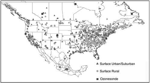
FIGURE 6-2 Locations of surface O3 monitoring sites and ozonesonde sites in North America. SOURCE: NARSTO 2000. Reprinted with permission; copyright 2000, EPRI, Palo Alto, CA.
Photochemical Assessment Monitoring Stations
The CAA Amendments of 1990 required EPA, in partnership with state and local agencies, to carry out more extensive monitoring of O3 and its precursors in areas with persistent exceedances of the O3 NAAQS (those O3 nonattainment areas that are classified as severe or worse). In response, EPA established a network of photochemical assessment monitoring stations (PAMS) in 24 urban areas (see Figure 6-3) to collect detailed data for VOCs, NOx, O3, and local meteorology. The chief objective of PAMS data collection is to provide an air quality database that will assist air pollution control agencies to assess and refine O3 control strategies and specifically to evaluate the trends in and effectiveness of controls implemented on VOC and NOx emissions in an area and to evaluate photochemical models being used by state and local agencies to carry out the attainment demonstrations required for their SIPs (see Chapter 3).
In principle, the data from the PAMS network could be extremely useful for the regulatory and scientific communities. However, it appears that the full potential of the data has yet to be realized (NARSTO 2000). Questions concerning the accuracy and specificity of the VOC and NOx concentrations obtained from the PAMS instrumentation have limited the ability of researchers to use the data to empirically assess the relationships between ambient VOC and NOx concentrations and O3 formation (Parrish et al. 1998; Cardelino and Chameides 2000). In spite of those limitations,
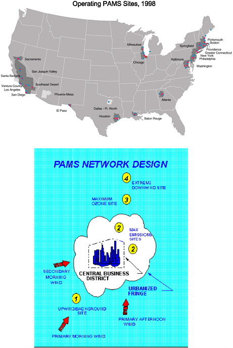
FIGURE 6-3 The PAMS network. Top Panel: Map showing the locations of PAMS sites in 1998. Lower Panel: A schematic showing the general design of the network within an urban area with upwind and downwind sites as well as sites near the largest sources of precursor emissions and sites where O3 concentrations are typically at a maximum. SOURCE: PAMS 2002.
the PAMS data sets can probably still be used to evaluate trends, but this type of evaluation generally requires a record of measurements of a decade or more, and the PAMS network is just now reaching that level of maturity.
Gaseous Pollutant Monitoring Program
Complementing the aforementioned urban-focused networks is the Gaseous Pollutant Monitoring Program (GPMP) operated by the U.S. National Park Service. The goal of this network is to provide data on baseline and trend concentrations of O3 and other pollutants in national parks, data that can be used to assist in the development of policies to protect park resources.
Interagency Monitoring of Protected Visual Environments
The Interagency Monitoring of Protected Visual Environments (IMPROVE) is a monitoring system established to assess visibility levels and trends and to identify sources of visibility impairment primarily in national parks and wilderness areas. Through the IMPROVE program, annual and seasonal spatial patterns in PM and light extinction can be assessed (Box 6-1).
|
BOX 6-1 Visibility impairment from air pollution arises primarily from the scattering and absorption of light by suspended particulate matter (PM) with an aerometric diameter less than 2.5 μm. The contribution of human activities to visibility impairment in wilderness areas and national parks is assessed by monitoring the concentration and composition of PM in these areas and deriving so-called light extinction coefficients and visibility ranges from these measurements. Visibility trends thus derived vary by region and are not fully intercomparable because of the infrequent PM sampling schedules typically used. In the eastern United States, visibility has shown some improvement in the last decade but remains seriously degraded. The mean visual range is about 24 kilometers (km), compared with visibility in a “pristine” atmosphere in the range of 75–150 km. In the western United States, visibility levels do not appear to have changed significantly in the past decade; the mean visual range is 80 km compared with natural visibility of 200–300 km. (Visibility is less in the eastern United States even in the absence of human activities because of the higher humidity, which enhances the ability of particles to scatter light.) There is evidence that over the period 1988–1998, visibility declined in some national parks because of area increases in sulfur emissions (Sisler and Malm 2000). As discussed in the preceding chapters, EPA adopted a new regional haze program in 1999 to help address this problem. |
Enhanced PM2.5 Monitoring Networks
Many of the monitoring networks described above have been collecting routine observations of airborne total suspended particulates (TSP) and PM10. However, with the promulgation of a new NAAQS for PM2.52 in 1997 came the need for a national monitoring program for PM2.5. The resulting network could be used to help meet four objectives: (1) establish locations of nonattainment of the PM2.5 NAAQS; (2) aid in the design of SIPs and then track their effectiveness; (3) assess regional haze and visibility (Box 6-1); and (4) provide data for health effects studies and other ambient aerosol research. Two types of measurements are undertaken in the network: (1) monitoring of the total mass concentration of PM2.5, and (2) determination of its chemical composition. The network, as currently designed, uses a filter-based technique to measure and characterize PM2.5. Particles from the atmosphere are first collected on filters by passing ambient air through them over a period of time (typically 24 hr), and the filters are then analyzed gravimetrically to determine PM2.5 mass concentration and chemically to determine PM2.5 composition. Although the filter-based technique is relatively straightforward for state and local agencies to implement, it is labor-intensive and subject to a variety of positive and negative artifacts, especially for the determination of chemical composition (Pierson et al. 1980; EPA 2002b). Although considerable progress has been made in eliminating these artifacts (for example, through the use of annular denuders, filter packs, and backup sorption beds), a number of problems remain unresolved. To enhance the long-term ability of the PM2.5 network to meet the needs of the regulatory, health effects, and air pollution research communities, those remaining problems will need to be addressed adequately, or other techniques less susceptible to artifacts will need to be deployed. A new class of semicontinuous PM monitors shows promise in this regard.
To address the problems with the filter-based techniques and to respond to the recommendations of the National Research Council (NRC 1998b, 1999a, 2001d), EPA has implemented a number of PM “supersites,” where more detailed research is addressing the scientific uncertainties associated with fine PM. Program goals focus on fine particulate characterization, methods testing, and support of studies of health effects and exposure. Locations of the initial PM supersites are shown in Table 6-3.
Hazardous Air Pollutants
There is not as extensive a nationwide monitoring network for hazardous air pollutants (HAPs) as there is for criteria pollutants. A large number
TABLE 6-3 Locations of Initial PM2.5 Supersites
|
Location |
Oversite Institution |
|
Baltimore, MD |
University of Maryland at College Park |
|
Fresno, CA |
Desert Research Institute and California Air Resources Board |
|
Houston, TX |
University of Texas at Austin |
|
Los Angeles, CA |
University of California at Los Angeles |
|
New York, NY |
State University of New York at Albany |
|
Pittsburgh, PA |
Carnegie Mellon University |
|
St. Louis, MO |
Washington University |
|
Atlanta, GA |
Georgia Institute of Technology |
|
SOURCE: Adapted from EPA 2002o. |
|
of HAPs are monitored at PAMS sites, and a number of local and state HAP monitoring programs are in place. These programs vary considerably from one location to the next in terms of the species measured, the types of localities monitored, and the frequency and quality of measurements (EPA 2000e; Kyle et al. 2001). Although the data needed to assess trends in HAPs are sparse, EPA has reported trends for a small subset of the most critical HAPs (Box 6-2). EPA is working to create a more consistent, comprehensive national monitoring network for a small set of HAPs. In 2001, it began a pilot monitoring project that includes 10 locations and an initial trends network that includes 11 cities. These trial efforts are aimed at helping to assess sampling and analysis precision requirements, sources of variability, and minimal detection levels.
Deposition Monitoring Networks
National Atmospheric Deposition Program and National Trends Network
Wet deposition of major solutes is monitored throughout the country by the interagency-supported National Atmospheric Deposition Program and National Trends Network (NADP/NTN) (see Figure 6-4). The primary aim of the network is to determine the exposure of natural and managed ecosystems to nutrient and toxic elements and acidity arising from anthropogenic activities, such as fossil fuel burning and agriculture. The spatial pattern of the wet deposition is estimated with a hybrid data-assimilation and modeling system that incorporates NADP/NTN data with information on spatial patterns of topography and precipitation. Application of this system appears to confirm that the aforementioned reductions in SO2 emissions from power plants achieved as a result of the Acid Rain Program of the 1990 CAA Amendments have resulted in a decrease in sulfate deposition in the eastern United States (Box 6-3). Moni-
|
BOX 6-2 EPA (2000d) estimates that the 1996 level of HAP emissions decreased by 23% compared with the 1990–1993 baseline period. It is difficult to confirm the accuracy of these emission-trend estimates using ambient data because of the short time span being considered and the limited coverage of monitoring sites. Nevertheless, EPA reported trends for 33 urban HAPs for the period 1993–1998 (EPA 2000d) based on existing data and found evidence of downward trends in the majority of HAPs being monitored. The greatest reductions were seen for benzene (Figure 6-5) and suspended lead, both due primarily to changes in fuel formulation that resulted in either substantial reduction in emissions (in the case of benzene) or their elimination (in the case of lead). (See Chapter 4 for a more detailed discussion of these efforts.) |
toring for current and future toxic air pollutants of concern in a consistent manner across the nation and in a way that provides data to support exposure and risk characterization is an important consideration, and research into methods to accurately estimate ambient concentrations and exposure to HAPs is needed.
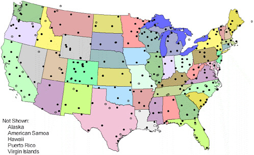
FIGURE 6-4 Locations of the National Atmospheric Deposition Program and National Trends Network (NADP/NTN) monitoring sites in the contiguous 48 United States. SOURCE: NADP/NTN 2002.
|
BOX 6-3 As a result of the application of continuous emissions monitoring (CEM) to utilities regulated under the acid rain provisions of the CAA, it is reliably estimated that annual SO2 emissions from utilities have declined by about 5 million tons during the 1990s (see Figure 5-1 in Chapter 5). The next step in an AQM assessment of progress is to ensure that these reductions in emissions produced the appropriate atmospheric response—a reduction in sulfate deposition rates. That reduction has occurred, as illustrated in Figure 6-6 and according to an analysis of data from the National Atmospheric Deposition Program and the National Trends Network (Stoddard et al. 2003). The final step is to determine if these reductions have led to the appropriate ecosystem response. This issue is discussed in Box 6-6. |
National Atmospheric Deposition Program and Mercury Deposition Network
The Mercury Deposition Network (MDN) was established as part of the NADP to measure wet deposition of total mercury (as well as methylmercury at some sites). The MDN is located mostly in the northeastern
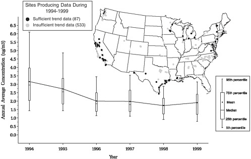
FIGURE 6-5 National trend in annual benzene concentrations in metropolitan areas, 1994–1999. SOURCE: EPA 2001a.

FIGURE 6-6 Trends in wet sulfate deposition in the United States using data from the Clean Air Status and Trends Network (CASTNet) and the National Atmospheric Deposition Program/National Trends Network (NADP/NTN) (1989–1991 vs. 1997–1999). Data are in kilograms per hectare. The largest decreases are indicated across the mid-Appalachians, the Ohio River Valley, and the Northeast regions of the country. SOURCE: EPA 2003o.
United States and is largely funded by state agencies. The long-term objective of the MDN is to assess national-scale spatial patterns and temporal trends in wet deposition of mercury. However, because the network has operated for only a few years on a small number of sites, it can only provide information on site-specific deposition.
Clean Air Status and Trends Network
The Clean Air Status and Trends Network (CASTNet) measures the components of atmospheric deposition that enter the environment in dry form, such as particles and gases. Monitoring dry deposition is critical in determining the total pollution load across the United States. For example, dry deposition in some areas contributes as much as 60% of the total sulfur deposition. Two-thirds of CASTNet sites are located east of the Mississippi River. Dry deposition rates are calculated using atmospheric concentrations, meteorological measurements, vegetation characteristics, land use, and surface conditions. Such factors impart a high amount of uncertainty to estimates of the spatial patterns of dry deposition. Therefore, regional patterns and long-term trends have not been well characterized.
Atmospheric Integrated Research Monitoring Network
The Atmospheric Integrated Research Monitoring Network (AIRMoN) provides highly resolved information over time on precipitation and dry deposition by using daily sampling methods. AIRMoN is designed to provide an intensive research-based foundation to support the routine operations of NADP and CASTNet. Whereas NADP and CASTNet are designed to characterize long-term trends, AIRMoN uses a small number of sites at selected locations to more quickly detect a temporal trend in deposition that might arise (for example, from emission controls or from new sources) and to evaluate the effects of these trends on sensitive ecosystems. There are currently two components of AIRMoN—7 sites to detect changes in wet deposition and 13 sites to evaluate changes in dry deposition. The flat funding for this program for 10 years has resulted in the closing of three dry deposition sites.
Air Quality Monitoring Discussion
The nation’s air quality monitoring system has evolved considerably over the past 30 years and will need to continue evolving to meet future air quality challenges. In this section, particular strengths, weaknesses, and other aspects of the air quality monitoring system are considered. EPA is developing a new national ambient air monitoring strategy, which includes a new network design called NCore, as well as a continuous monitoring implementation plan. The report outlining these new plans has been released in draft form and is undergoing review by state and local agencies and the academic and technical communities (EPA 2002p). The committee did not assess the extent to which these plans will help address the concerns discussed below.
Monitoring Objectives
Monitoring networks are an essential part of any air quality management system and can help to meet one or more of the following objectives (Chow et al. 2002a,b; Demerjian 2000; NARSTO 2003):
-
Determine the specific air pollutants or their mixtures that are associated with health and welfare effects, including visibility impairment.
-
Estimate exposure of human populations or sensitive ecosystems.
-
Measure compliance with ambient air quality standards.
-
Develop information about the sources contributing to the pollution.
-
Develop information on processes controlling the formation, removal, and transport of the various pollutants and their precursors.
-
Measure the effectiveness of emission-control programs.
-
Serve as a warning system to alert individuals that are sensitive to poor air quality and to aid in the development of air quality forecasts.
Each one of the objectives places different demands on a network in terms of the species measured, instrument sensitivity, time resolution and frequency of the measurements, and location of the monitoring stations. Even though more than $200 million per year is spent on routine air quality monitoring in the United States (EPA 2002p), monitoring networks have limited resources. As a result, they are able to address only some of the above objectives adequately. At least two major issues arise as a result of resource limitations (NARSTO 2000):
-
Identifying the problem versus finding the solution and assessing program effectiveness. Most of the existing networks have been designed only to measure compliance with the existing NAAQS and reveal little about the appropriate management strategies needed to solve the problems or measure the success of various emission-control strategies (see earlier discussion on emission trends). Network design should be evaluated and expanded to make air quality networks in the United States more relevant to other important objectives of monitoring. Some specific changes are discussed below.
-
Measuring critical species in a regular monitoring mode. Because of the variety of criteria pollutants, their precursors, and HAPs and their large range of concentrations, monitoring is technically challenging as well as expensive. In some cases, these challenges are beyond the capabilities of state and local regulatory agencies. Creative mechanisms for fostering collaboration and technology transfer among regulatory agencies, research and academic institutions, and small businesses need to be devised to meet the challenges (see discussion in Box 7-5 in Chapter 7).
Siting of Air Quality Monitoring Stations
Following enactment of the CAA, the AQM system in the United States emphasized urban-scale air quality problems and the use of controls on local emissions to solve air pollution. Moreover, major urban areas were the only areas specifically identified in the congressional mandate that initially directed the EPA administrator to develop a national monitoring program. As a result, the nation’s ambient air quality monitoring networks have been dominated by urban sites. The intervening years have seen a growing concern for large-scale air quality problems that extend over multistate airsheds and are affected by long-range transport. However, a
concomitant evolution of the nation’s air quality networks has not occurred for gaseous pollutants. For example, NAMS and SLAMS for O3 contain about 1,600 sites. Those that are urban and suburban sites outnumber rural sites by a factor of 2 (see Table 6-4).
The largely urban-based networks in use in the United States have proved quite useful for characterizing urban air quality for the specified pollutants; however, there are several limitations to the information that can be gained from these networks. In particular, they are inadequate for characterizing air quality on a regional scale; they provide little information to address processes related to the production of secondary pollutants, such as O3; and the spatial coverage of these data is relatively small and not well suited for use in air quality model performance evaluation. Moreover, to assess urban emission impacts, many of the so-called rural sites are located within or directly downwind of urban areas and are therefore often affected by urban pollution plumes (NARSTO 2000). The sites in PAMS, the other major network for gaseous pollutants, are also by congressional mandate exclusively located in and around major metropolitan areas (see Figure 6-3). The current lack of rural monitoring sites severely hampers the AQM system’s ability to address multistate airshed pollution problems or to assess and mitigate pollutant impacts on natural and managed ecosystems, such as agriculture. It also may hamper the ability to identify the true extent of NAAQS nonattainment. For example, analysis of monitoring data from rural areas suggests that a large fraction of rural counties in the eastern United States might be in violation of the new 8-hr O3 NAAQS (Chameides et al. 1997). It is not possible, however, to assess the extent of this rural nonattainment without more extensive rural monitoring.
Another shortcoming of the current monitoring networks for gaseous and aerosol pollutants is their strong emphasis on measuring ambient concentrations rather than concentrations in specific microenvironments that
TABLE 6-4 Ozone Monitoring Sites in the United Statesa
may sometimes be hot spots.3 In the absence of data on pollutant concentrations in hot spots, characterization of pollutant exposures of persons who work in, reside in, or travel through them is problematic (see Box 7-5 in Chapter 7).
Air Quality Measurement Techniques
Standard operating procedures, measurement methods, and quality assurance and quality control (QA/QC) procedures are critical to ensure that the data sets from monitoring networks can be directly compared and integrated for use in trends analysis, for investigations of atmospheric processes, and for improvement of predictive models. In accordance with the Code of Federal Regulations (40 CFR Part 53 [2002]), EPA established federal reference methods (FRM) and federal equivalent methods (FEM) to be used in measurements of criteria pollutants (EPA 2002q). Further development of monitoring techniques is needed, however, to address some of the following concerns:
-
The instrumentation used to measure NO and NO2 in the FRM does not have the sensitivity or the specificity to measure nitrogen oxides accurately over the full range of conditions typically encountered by such instrumentation (McClenny et al. 2002).
-
PM10 and PM2.5 are generally measured once every 3 or 6 days, a sampling rate that is too infrequent to capture the true variability of PM concentrations.
-
New analysis systems were developed in response to the PAMS initiative and its requirements for measurements of speciated hydrocarbons and carbonyl compounds. However, routine monitoring of hydrocarbons and carbonyls is a challenging task, even for research institutions, and thus far, delivery and analysis of quality-ensured data from PAMS have been limited (see NARSTO 2000).
-
PM2.5 measurements will continue to pose a technical challenge because of the complex multiphase mix of constituents in ambient aerosols. As noted earlier, current sampling methods are subject to various artifacts.
-
For example, nitric acid and organic vapors may adsorb on the filter used for the collection of atmospheric particles (positive artifacts), and ammonium nitrate or organic PM may evaporate from the filter during sampling (negative artifacts). Many studies have been completed or are being conducted to develop and test more reliable monitoring methods and analytical procedures to determine the chemical composition of PM (see NARSTO [2003] for a review). A promising new technology based on automated semicontinuous sampling technology has been developed in the supersites programs and could be used in the routine Speciation Monitoring Network.
-
There is an emerging interest in bioaerosols—fine PM of biological origin, which may include allergens, viruses, bacteria, or fungi. They can enter the atmosphere inadvertently as a result of animal-feeding operations (NRC 2003c) or intentionally as a result of bioterrorism (NRC 2002d). Identification of these materials will be more complex than simple chemical or elemental analysis and may involve microbiological tests.
-
Because the primary focus of monitoring strategies has been on documenting NAAQS attainment, there is little motivation to develop methods to measure ambient concentrations that are substantially below the standards. Such measurements are needed to provide critical data for understanding atmospheric processes and providing input for air quality models.
Air Quality Trend Analysis Techniques
A variety of techniques can be used to determine long-term trends in ambient pollutant concentrations. The method most commonly used by EPA is to compute yearly averages of concentrations at all stations within a metropolitan statistical area (MSA). Values for missing yearly averages are linearly interpolated if in a middle point; missing end points are replaced with the nearest year of valid data. Linear regression analysis is done, and a method known as the Theil test (Hollander and Wolfe 1973) is applied to detect the significance of any trend. This approach is a fairly simple, straightforward method of trend detection, but it has several important limitations. As noted earlier, the monitoring stations may not be, and often are not, spatially distributed to document the average air quality over the region of interest, and thus the trends derived might not be representative of the region. The results of a linear regression analysis can be highly sensitive to such factors as the time interval chosen for analysis and the frequency of observations. In some cases, sparse data make it difficult to calculate trends. For instance, samples of PM are generally collected at a frequency that is longer than most PM episodes. Consequently, several years of data collection will be needed to characterize seasonal and spatial patterns accurately and an even longer period of sampling will be needed to detect long-term temporal trends.
One of the greatest challenges in concentration trend analysis—carried out with the specific purpose of determining if pollution control efforts have been successful—is accounting for meteorological influences, which can cause a great deal of variability in concentrations and are often large enough to obscure changes in anthropogenic emissions. A variety of statistical approaches (such as regression-based modeling and extreme value approaches) can be used to filter out meteorological influences from a trend; however, the results often vary, depending on the method and the specific concentration metric used.4 For all these reasons, most pollutant concentration trends cited by EPA and other organizations (including the trends noted in this report) should be used with caution (Box 6-4).
Data Availability
EPA issues a yearly National Air Quality and Emission Trends Report (EPA 2000e), which provides a general summary of the nation’s air quality. The summary includes the results of an analysis of air pollutant trends based on data obtained from the monitoring networks described above. EPA also issues a yearly Toxics Release Inventory (TRI) (EPA 2003m), which contains information about the types and amounts of approximately 650 chemicals that are released from certain industries and federal facilities. The reported information includes annual estimates of emissions as well as releases to water and land and quantities of chemicals sent to other facilities for waste management. However, the trends reports and TRI reports are intended for a general audience and do not contain enough information to facilitate more extensive analyses by the scientific and technical community. For such purposes, EPA has developed the Aerometric Information Retrieval System (AIRS), a framework that provides access to monitoring data from different sources. Although EPA has made efforts to update AIRS, problems remain with the system that limit its utility. All monitoring data are not stored in AIRS, and data stored in AIRS have not been “standardized”; for example, the data have not been converted to uniform measuring units or to universal standard time. Most important, the data are not available in real time (as are, for instance, data from the National Weather Service). Although EPA maintains the AIRNow web site where individuals can access information on present and past air quality conditions at localities throughout the United States, the information is qualitative and thus not suitable for quantitative analyses. Many states have begun to make their air quality monitoring data available in real time over the
|
BOX 6-4 EPA analyses show that over the past 20 years, national 1-hr average O3 concentrations have decreased by about 18%; most major metropolitan areas showed downward tends, and the Northeast and West showed the greatest improvements. In contrast, the South and North-central regions of the country and many national parks show increased O3 concentrations over the past 10 years. However, numerous uncertainties are associated with those O3 trend estimates. The formation and accumulation of O3 are strongly affected by prevailing meteorological conditions. Therefore, O3 trends, driven by emission-control policies, can be easily masked by year-to-year meteorological variability, and trend analyses can reach very different conclusions based on the methods used to factor out meteorological influences. O3 trends have been routinely examined using the second highest daily maximum 1-hr average concentration in a given year, because that value is used to establish compliance with the 1-hr O3 NAAQS; however, that value tends to fluctuate with a larger amplitude than a more robust statistic, such as the 95th percentile. As a result, subtle trends can be masked by the fluctuations of the extreme values. Several research groups have questioned EPA’s reported O3 trends and carried out independent studies using data from national monitoring networks. A comprehensive review of such studies is presented by Wolff et al. (2001). Some locations, such as Los Angeles, have shown consistently decreasing O3 trends, but national-scale studies paint a more complicated picture. Milanchus et al. (1998) examined daily maximum 1-hr O3 concentrations over the period 1984–1995 and found that most locations exhibited downward trends during that time, and a few isolated sites showed upward trends. Fiore et al. (1998) examined median summer afternoon O3 concentrations for the years 1980–1995 and found that trends were insignificant over most of the continental United States, although O3 concentrations decreased in New York, Los Angeles, and Chicago. A follow-up study examined trends in the number of exceedances of the O3 standards (Lin et al. 2001). Over the period 1980 to 1998, strong downward trends in the number of days in exceedance of either O3 standard were found along the northeastern and southwestern coasts, and significant upward trends were found in various locations elsewhere in the country. In most locations, the O3 air quality improvements seen in the 1980s leveled off in the 1990s. The results differ among those and other studies because they are based on different yearly ranges, time periods within each year, pollution metrics, and methods to account for meteorological effects. Thus, it is very difficult to compare and evaluate the validity of reported O3 trends systematically based on past analyses. |
internet. That is an important development that should be encouraged at the national level by EPA. The availability of air quality data in real time will open up significant entrepreneurial and research opportunities. For example, real-time air quality data could greatly facilitate the development of predictive (4-dimensional data assimilation) air quality modeling systems that could be used to assist air pollution mitigation efforts (Box 6-5).
|
BOX 6-5 The role of air pollution forecasts is growing as an AQM tool. Most forecasts produce 1–3-day O3 forecasts that predict exceedances of specific concentration thresholds. These forecasts can be used as a warning system for individuals sensitive to poor air quality and as an AQM tool. The techniques used to make these forecasts usually fall into one of four general types (Dye et al. 2000; NOAA 2001):
Although air pollution forecasting for secondary pollutants, such as O3, is a relatively new scientific endeavor, and the accuracy and predictive skill of the methods described above have yet to be evaluated comprehensively (NRC 2001a), such forecasting has begun to be used in an operational mode. In some instances, predictions of future air pollution episodes are released to the public as an advisory. Individuals, especially those most sensitive to air pollution, can, if they choose, use the information from these advisories to alter their behavior in a way that would minimize their exposure to the pollution. For example, in AIRNow, probably the largest national air pollution forecasting effort, EPA provides the public with same-day and next-day O3 forecasts as well as PM2.5 forecasts for many cities. The AIRNow program developed an infrastructure to collect daily air quality forecasts from state and local agencies for over 250 cities and provide real-time and forecasted air quality data to the public through media outlets (Wayland et al. 2002). EPA compiles air quality forecasts and posts them to the AIRNow website for public utilization (www.epa.gov/airnow). |
|
Similarly, the National Weather Service (NWS) intends to develop and implement a nationwide system for distributing air quality forecasts in conjunction with NOAA’s Office of Oceanic and Atmospheric Research, EPA, and the air quality modeling community to provide to the public information such as current ozone conditions from live weather broadcasts (Stockwell et al. 2002). NOAA has also developed several experimental forecast products (including models to predict smoke dispersion from forest fires) and made them available on the internet, and the National Park Service has begun to issue O3 advisories for some national parks to protect its workforce and to alert park visitors. In more ambitious operational applications, air pollution predictions are used by air quality managers to trigger specific emission reductions—that is, temporary measures to lower pollutant emissions to avert or at least limit the severity of the episode. A growing number of state and local air quality agencies are using summertime O3 forecasts to take steps to reduce precursor emissions. Many cities now use forecasts to declare “ozone action days,” when the public is encouraged on a voluntary basis to modify their activities to reduce O3-producing emissions. To date, their effectiveness has not been independently evaluated. From a technical point of view, a major concern of the growing use of air pollution forecasting as an operational tool is the apparent lack of a concomitant effort to design and implement tools to assess the accuracy of the forecasts and the impact their use has on averting adverse health effects and reducing pollutant emissions. If air pollution forecasting is to reach a level of sophistication and use comparable to that of meteorological forecasting, a serious program of assessment must be undertaken. |
Monitoring Vertical Profiles of Air Pollutants
Vertical profiles of pollutants are only available from intensive, research-oriented field campaigns and thus are very limited in time and space. Results from several observational campaigns in the United States and abroad have demonstrated the importance of making vertical measurements of pollutants (see Kleinman and Daum 1991; Berkowitz et al. 1996; Hamonou et al. 1999; Simo and Pedros-Alio 1999; Ansmann et al. 2000). A variety of techniques can be used routinely to measure vertical profiles of atmospheric composition and related meteorological variables, including use of aircraft, which can provide a valuable platform for studying atmospheric composition over a wide range of altitudes. Kleinman and Daum (1991) studied the vertical distributions of airborne particles, water vapor, and insoluble gases in measurements taken during aircraft flights conducted near Columbus, Ohio, and found plumelike features at high altitude where pollutant concentrations increased by 50% or more for distances of several kilometers. These features were attributed to air near the earth’s surface lofted by convective storms. These types of studies are important in quantifying the role of long-range transport (see next section), because pollutants that have
been lofted above the boundary layer will travel farther from their sources, and in better elucidating the relationship between pollution and meteorological conditions.
High-resolution vertical profiles of pollution plumes aloft can also be obtained with balloon-borne instruments called ozonesondes that measure concentrations with an electrochemical cell. For example, the National Oceanic and Atmospheric Administration’s (NOAA) Climate Monitoring and Diagnostics Laboratory (CMDL) has a network of eight sites that make weekly O3 vertical profile observations from the surface to about 35 kilometers (km) (NOAA 2003). In addition, differential absorption lidars (a laser-based instrument that measures the light backscattered by particles along the beam path) can be used to obtain vertical profiles of atmospheric constituents.
Monitoring Long-Distance Transport of Air Pollutants
As state and local emission controls have successfully reduced local pollution sources, long-range transport has become an increasingly important source of NAAQS violations, especially for O3 and PM2.5. Yet, very few air quality monitoring sites allow meaningful examination of long-range pollution transport. Additional monitoring sites located outside urban areas provide important information for developing effective regional control strategies and would be an important element in helping to implement recommendations made in Chapter 7. However, current ground-based networks are inadequate for a quantitative determination of long-range pollutant transport, as much of it occurs above the boundary layer. Some additional information on long-range transport can be gleaned from high-elevation rural monitoring sites. Over the longer term, satellite remote-sensing techniques have the potential for comprehensively monitoring pollutant transport on regional and global scales. For example, Fishman et al. (2003) have used satellite-based instruments to provide detailed maps of tropospheric O3 that are capable of defining the regional extent of O3 pollution in areas around the world. Current satellite instruments can provide a qualitative picture of the atmospheric distribution of some aerosol types, but quantitative information on aerosol type and mass flux is difficult to obtain because of the poorly characterized radiative properties of most aerosols (NRC 2001a).
ASSESSING HEALTH BENEFITS FROM IMPROVED AIR QUALITY
A primary goal of the nation’s AQM system is the protection of human health. Therefore, an important aspect of measuring progress in AQM is demonstrating that reductions in pollutant emissions and improvements in
air quality have resulted in measurable health benefits or that preventative measures have averted a worsening of public health. Such a demonstration not only helps to confirm that the appropriate air pollutants are being regulated but also helps to establish that the societal expenditures made to improve air quality have benefited society directly and concretely. Although the process of setting goals and standards discussed in Chapter 2 has much in common with the process of assessing health benefits from improved air quality, they are two distinctly different and independent activities. The former identifies adverse effects and risks and sets goals and standards to avoid or decrease these effects and risks; the latter establishes retrospectively that specific improvements in air quality have resulted in a reduction in adverse health effects.
Ideally, an analysis of the benefits of air pollution mitigation for public health would rely on independent toxicological and epidemiological data that linked specific long-term air pollution trends with specific trends in public health. However such linking has proved to be particularly difficult (EPA 2003n). Although there is a wealth of overlapping data on temporal patterns of disease within specific populations and on patterns of air pollution in areas where the population resides and/or works, air pollution is believed to account for a small proportion of the current incidence of disease in the United States (HEI 2000). Changes in other risk factors, such as age, socioeconomic status, amount of smoking, occupation, and weather, whose distribution and effect in the population can vary over time, can easily mask any benefits related to air quality improvements. For example, the potential for reduced exacerbation of asthma due to reductions in air pollution might pose an opportunity to track actual health benefits. Associations of PM with exacerbations of asthma have been repeatedly demonstrated epidemiologically in time-series analyses of emergency-room visits and hospital admissions and in panel studies examining associations with peak flow, medication use, and symptoms (Ostro et al. 1998). However, the underlying prevalence of asthma has increased significantly, especially among children, complicating efforts to track changes in asthma exacerbation in relation to changes in air pollution (for example, by looking at the number of asthma hospitalizations). Even if air pollution is declining, the size of the potentially vulnerable population is increasing, and the absolute number of hospitalizations might rise even as levels of pollution fall. This challenge is made even more daunting when one tries to track changes in multipollutant, multipathway exposures and the resulting changes in health.
Because of the current inability to directly link observed population health trends with contemporaneous ambient air quality benefits, less direct approaches have been adopted to assess the health benefits of reductions in air pollution. Aspects of three such approaches are discussed below.
Assessments Based on Data from Short-Term Air Pollution Events
Extreme air pollution events, such as those experienced in London, England, in the 1950s and 1960s, provide distinctive data sets linking the effects of such events with population health. For example, one of the most infamous air pollution events occurred in December 1952, in which air pollution dramatically increased over a 10-day period with a coincident large increase in cardiorespiratory disease, manifested by increases in hospital admissions and a doubling of the daily mortality. The number of daily deaths declined when air quality improved, albeit in a time-lagged manner (U.K. Ministry of Health 1954).
A related approach uses data from specific events that caused a temporary cessation of air pollutant emissions to establish a link between improvements in air quality and human health outcomes. For example, Friedman et al. (2001) found a significant statistical correlation between closure of inner city Atlanta to traffic during the 1996 Olympics and reduced visits to emergency departments for asthma in children. Similarly, Ransom and Pope (1995) used data from Utah Valley during two intervals in the late 1990s, when a steel mill was shut down due to a labor dispute, to characterize the relationship between PM10 concentrations and the incidence of bronchitis and asthma.
Data from extreme and short-term events can demonstrate the link between air pollution and adverse health effects as well as the ameliorative power of improved air quality. However, the data are only marginally relevant to the assessment of health benefits that accrue from gradual changes in pollutant concentrations expected under a broad, incremental program to control air pollution.
Assessments Using Risk Functions and Exposure Estimates
A second type of assessment method used by EPA in its examination of the health benefits of the CAA combines “risk functions” derived from the health effects literature and data from air quality monitors to estimate public health benefits (EPA 1997). The risk function is an estimate of the incremental change in a health indicator, such as daily mortality, hospital admissions, emergency-room visits, restricted-activity days, respiratory-symptom days, and asthma attacks, that results from an incremental change in the concentration of an air pollutant (or mix of air pollutants). This risk function is then multiplied by the observed change in ambient air pollution over some span of time using data from air quality monitoring (or estimates of emission reductions) to estimate the resulting change in the number of adverse health events.
The risk-function approach is widely used by the regulatory and public policy communities. For example, it has formed the basis for most of EPA’s
estimates of the health benefits of AQM in the United States (EPA 1996a). However, this approach has at least two potential pitfalls: (1) the trends in ambient air pollution derived from air quality monitors may not be representative of the actual trend in population exposure to pollution; and (2) the cause-and-effect link between improved air quality and improved public health is not directly measured. With respect to the second point, because the studies used to derive the risk functions can be the same as, or similar to, those used in the goal and standard setting process, this type of assessment does not provide an independent verification that the air quality improvements attained by an AQM system had the intended health benefits. Despite these limitations, the risk-function approach has the advantage of providing a relatively simple and straightforward method for translating observed changes in air quality into an associated health outcome and as such will likely continue to be used. Some specific measures that could be taken to improve the estimates derived using this approach are discussed below.
Assessments Based on Tracking Public Health Status and Criteria Pollutant Risk over Time
There have been a number of epidemiological studies throughout the world directly linking daily variations in PM with either mortality or hospitalization for heart and lung problems. The results of these studies provide a direct assessment of some of the population health impacts of ambient PM for specific locations and time periods. To date, however, there have not been consistent efforts to track health changes over time and to relate those changes to changes in air quality.
There are some indicators of pollution levels in the United States that have been and are being tracked over long periods (for example, EPA’s AIRS database for ambient pollutants). However, except for the National Death Index and Cancer Registry, there is no national tracking system for the full range of acute and chronic disease and associated environmental risk factors. Requirements for environmental health tracking are not consistent among the various state and local registries that are in use for chronic disease (EHTPT 2000), making it difficult to draw robust conclusions linking chronic disease clusters to environmental factors beyond local or state boundaries. Several programs are in place that can potentially be expanded or modified to provide a coordinated approach that identifies hazards and clusters of disease occurrences, evaluates exposure and environmental factors, and tracks the overall population health. These programs are the following:
-
The Pew Environmental Health Commission examined a number of national health outcome databases for information on chronic diseases
-
linked to environmental factors. These databases included the National Hospital Discharge Survey, the National Ambulatory Medical Center Survey, and the National Hospital Ambulatory Medical Care Survey. All provide information on patient demographics and health-care services administered, but they are not designed to describe the communities in which the illness occurred or the environmentally related health outcomes (EHTPT 2000).
-
The Centers for Disease Control and Prevention (CDC) Environmental Health Laboratory has an ongoing study to evaluate human exposure to environmental contaminants. Blood and urine samples are collected from a subset of participants from the larger NHANES5 effort and are tested for a range of environmental contaminants.
-
The National Children’s Study (NCS 2002), now in development, is designed to track the health of 100,000 children, starting at a prenatal stage and continuing into the adult years. The study includes tracking environmental factors, such as chemical exposures and nutrition, but does not monitor chronic diseases that may develop in the later years of life.
In addition, Congress provided CDC with funding in fiscal year 2002 of over $17 million to begin developing a nationwide environmental public health tracking network and to further develop capabilities to track environmentally related health problems within state and local health departments. CDC’s (2003a) goal is to develop a tracking system that integrates data on environmental hazards and exposures with data on diseases that are possibly linked to the environment to do the following:
-
Monitor and distribute information about environmental hazards and disease trends.
-
Advance research on possible linkages between environmental hazards and disease.
-
Develop, implement, and evaluate regulatory and public health actions to prevent or control environmentally related diseases.
With this appropriation, CDC funded 17 states, 3 local health departments, and 3 schools of public health to begin developing such a tracking network and state and local capabilities. Congress also is considering a broader bill entitled the Nationwide Health Tracking Act to develop a comprehensive system for identifying and monitoring chronic diseases and potentially correlating their causes with environmental, behavioral,
socioeconomic, and demographic risk factors. The information gathered from such a program could be used as a basis for taking steps to alleviate the sources of the disease affecting a particular community or the population as a whole.
There are a number of ways that an improved national health database, when coupled with ambient air quality data, could be used to derive a metric for the effects of AQM on health outcomes. For example, periodic epidemiological studies could be carried out that independently test for the association between ambient pollutant concentrations and the incidence of adverse health effects (Burnett et al. in press). If, over the course of the studies, the association between health outcomes and PM concentrations remained constant while PM concentrations declined, the association between the two would likely be robust and could be used along with the ambient data to directly estimate the premature deaths or hospitalizations avoided as a result of the air quality improvements. If the association changed—suggesting either a stronger or weaker association between air pollution and health—the indication would be that AQM actions taken changed the pollution mix to make it less or more toxic and that more analysis was needed before the actual health benefits accrued from AQM could be assessed. Although this approach is relatively new and has not been fully tested, it is encouraging to note that a similar approach was recently applied to analyzing health trends following an Irish government action to ban the use of coal in homes in Dublin, and a measurable improvement in premature mortality was observed (Clancy et al. 2002).
The development of these and other new approaches is indicative of the need perceived by the health effects research community to measure health changes more directly as air quality improves. This information could be used to hold air pollution regulations “accountable” for their health performance and to confirm that the improvement projected by new regulations actually occur. Several new initiatives are under way to develop these approaches further—for example, EPA is developing scientifically rigorous environmental indicators that can be tracked over time (Whitman 2001), and the Health Effects Institute is funding the development and testing of a variety of such techniques (HEI 2002).
Efforts to Track the Effects of HAP Emission Reductions
The challenges for assessing progress in health improvement as a result of reductions in emissions of HAPs are daunting, probably more so than those associated with criteria pollutants. As discussed above, the absence of a comprehensive air monitoring network for even a subset of HAPs makes direct measurement of long-term changes in exposure impossible (although recent efforts are attempting to fill that void). In addition, unlike
the criteria pollutants for which much of the health effects data provide evidence of relatively short-term, measurable changes in health, a major focus of HAP effects is cancer, which has long latency periods, making short-term tracking less fruitful. For example, recent reductions in benzene exposure might not result in measurable changes in cancers for decades. As a result of these limitations, EPA declined to provide an analysis on HAPs in its 1997 report to Congress on the benefits and costs of the CAA (EPA 1997).
Despite these challenges, there have been a number of efforts to develop baseline cancer risk estimates and hazard index calculations using dose-response information and exposure estimates derived from EPA’s 1990 cumulative exposure project (Axelrad et al. 1999) and similar projects. Cancer risk is estimated as the potency of the substance multiplied by an average daily dose. For substances assumed to have a threshold dose (below which health effects are not expected), exposure measures are compared with a reference concentration. Cumulative hazard index is the sum of ratios of pollutant exposure estimates to reference levels. These efforts are analogous in some ways to the baseline estimates for criteria pollutants used to justify regulatory action under the NAAQS and at least provide a start for future assessments as changes in HAP emissions are implemented.
The largest of these efforts is EPA’s National Air Toxics Assessment (NATA) (EPA 2002e), which characterizes inhalation risks from exposures to HAPs identified in the urban air toxics strategy (EPA 2000b) and from exposures to particles in diesel exhaust. NATA has provided a tool for exploring control priorities and has served as a preliminary attempt to establish a baseline for tracking progress in reducing HAP emissions. NATA provided estimates for the year 1996 and attempted systematically to evaluate and link emissions, ambient measurements, atmospheric transport, and human exposure. The main components of the assessment were the list of urban air toxics (EPA 2000b), the 1996 national toxics inventory of emissions, the Assessment System for Population Exposure Nationwide (ASPEN) dispersion model for developing estimates of ambient concentrations of HAPs from stationary emissions, the hazardous pollutant exposure model for developing exposure estimates for vehicular HAPs, microenvironment factors to establish the relationship between ambient concentrations and microenvironments of interest, toxicity metrics relating exposure to risk, and risk assessment guidelines providing further guidance on estimating risks from exposures.
A number of preliminary findings were of interest. Twenty-three of the 33 HAPs analyzed were estimated to present risks greater than 1 excess cancer incident in 1 million people, a risk threshold noted in several portions of Section 112 of the CAA. Major and area stationary-source emissions and on-road and nonroad mobile emissions were each associated with
risks of concern. A number of caveats were noted by EPA, indicating undercharacterization of risk and identifying major future research and data needs. For example, higher localized risks were not captured, and comparison of a national impact assessment with local impact assessments suggests underestimation for certain microenvironments in both urban and rural areas by factors of 30 and 100, respectively. Further, NATA’s attempts to compare modeling results with ambient data found the model underpredicted ambient exposures to some metals by a factor of 5. The tendency toward underestimation has been suggested to be due to gaps in the emissions inventory, but reductions in pollution releases since 1996 have effectively reduced the significance of these gaps, increasing the consistency between NATA estimates and current monitoring data (Environmental Defense 2002). Observed ambient concentrations of benzene were slightly underpredicted by the models, reflecting a lack of understanding of the emissions and environmental behavior of this compound. The assessment did not address dioxins, indoor air exposures, or noninhalation pathways. It also made no adjustments for other HAPs not listed in EPA’s urban air toxics strategy.
EPA (2002r) and the EPA Science Advisory Board (EPA/SAB 2001) have acknowledged that the current NATA effort has many limitations. In the absence of systematic monitoring of HAPs and the large gaps in personal HAPs exposure data, no comprehensive validation of the NATA models has been done. Although the health risk data for the compounds vary in quality, the estimates of cancer and other risks continue to be limited by the lack of a robust human database that avoids some of the challenges of extrapolation from higher concentrations. In its urban air toxics strategy, EPA is funding work to improve both the health database and the NATA. Pilot monitoring projects have been initiated to better characterize trends in ambient concentrations and to generate information on the temporal and spatial variability of ambient HAP concentrations (STAPPA/ALAPCO/EPA 2001). These efforts will likely address some of the pressing problems associated with tracking health impacts from HAPs; however, the remaining data gaps are significant.
Other HAP Assessments
In addition to NATA, there have been a number of conceptually similar assessments of HAPs, although none has evaluated trends at the national level. These assessments have included the following:
-
Cancer and noncancer HAP risks calculated as part of EPA’s comparative risk project were considered sufficiently serious (relative to risks addressed by other EPA programs) to rate HAPs as high risk (EPA 1987).
-
The California South Coast Air Quality Management District completed an assessment of trends in cancer risk from the mid-1980s to 1997 on the basis of a monitoring and modeling effort for 20 HAPs. The multiple air toxics exposure study (MATES II) used traditional techniques to study urban HAPs in California’s South Coast Air Basin (encompassing Los Angeles, Riverside, Orange, and San Bernardino counties) (SCAQMD 2000).
-
An assessment for Minnesota estimated exposure to 148 HAPs from EPA’s 1990 cumulative exposure project. Relatively high concentrations were found in the St. Paul metropolitan area and many smaller cities throughout the state.
-
The California Comparative Risk Project (CCRP) established risks of high concern for a number of HAPs, especially when more highly exposed populations were addressed (CCRP 1994). A more recent attempt to use monitoring data to conduct a comprehensive evaluation of the impact of HAPs noted the paucity of toxicity measures for many HAPs and the limited monitoring data for HAPs in California, a state with one of the most extensive monitoring networks. It was concluded that the information necessary to assess fully the health significance of HAPs was not available (Kyle et al. 2001).
Tracking Progress in Reducing HAPs-Related Health Effects for the Future
In summary, the ability to assess changes in health related to reductions in HAP emissions has been limited by the absence of high-quality data on ambient concentrations, the limitations in the health database, and the challenges of tracking health progress for diseases, such as cancer, that have long latency periods. Over the past decade, EPA and others have made strides to improve the techniques available for such assessments, most notably through the recent development of NATA. Both that assessment and the urban air toxics strategy noted limitations in the current analyses and the steps needed to be taken to improve them. Over time and with better air quality data, improved validation of exposure models, and enhanced health understandings, these techniques will track progress much more directly than those used today. Implementation of these efforts will require sustained attention and resources over the coming decades.
Monitoring Actual Human Exposure
AQM progress can be also be evaluated by directly tracking human exposure to air pollutants over time. Because concentrations measured by ambient monitors may not reflect human exposures, personal monitors worn by study participants have been used, and sampling of biomarkers in,
for example, blood and breast milk has been done. Corresponding environmental samples provide information on source contribution (for example, ambient air, indoor air, and food) (EPA 2002s). EPA has initiated the National Human Exposure Assessment Survey (NHEXAS) to document status and trends of national distributions of human exposure, and to that end, EPA has begun a series of pilot projects. A stated objective is to evaluate the efficiency of EPA’s regulations to reduce exposure. NHEXAS attempts to evaluate total human exposure to chemicals of concern and from contributions from different sources (see, for example, Clayton et al. 2002). Personal air monitors measure air breathed by individuals, diet and other samples are taken to address other routes of exposure, and blood and urine samples are obtained to characterize total exposure. An exploratory study under NHEXAS also evaluated selected subpopulations that might exhibit higher exposures (Pellizzari et al. 1999).
Methods using biomarkers as a surrogate for exposure to air pollution and other sources of environmental stress are developing rapidly and have great promise. Human biomarkers of air pollution are specific compounds or cellular changes that appear within the body, indicating the occurrence of exposure and a stress-related response to a specific pollutant or set of pollutants. These biomarkers can be the pollutant itself, one of its metabolites, or an enzyme produced in response to the pollutant or its metabolites. They can also be specific for modification of DNA (for example, DNA adducts). Biomarkers can potentially appear in blood, urine, or a specific organ where a pollutant might accumulate or do damage.
Because exposure biomarkers are a specific indication of exposure and a primary step in the causal chain of a disease outcome, their appearance provides stronger evidence of an actual health outcome from exposure to a pollutant compared with measurements of ambient pollutant concentrations. As such, tracking the appearance and abundance of specific biomarkers within a population over time may be a useful and convincing way to document a public health benefit (or lack thereof) from air quality improvements. Risk functions based on the presence and concentration of a given biomarker can then be used to estimate specific health changes more reliably. A classic example of the utility of this approach is the study linking decreases in Pb emissions from mobile sources to declining concentrations of Pb in ambient air and human blood (see Figure 6-7A-C). A recent CDC report illustrated another example: a measurable decline in the levels of cotinine—a marker for exposure to environmental tobacco smoke—in a random sample of the U.S. population found in tracking the increasing restrictions on smoking in public spaces (CDC 2001).
However, the development of compound-specific markers of actual effects or early stages of effects has been much more difficult. To date, several compound-specific markers of exposure have been developed (for
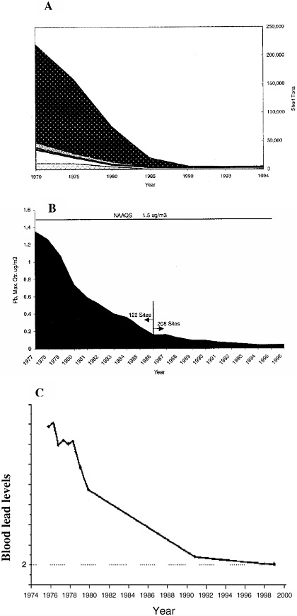
FIGURE 6-7 (A) Total estimated U.S. lead emissions by major source category from 1970 to 1994. (B) Maximum quarterly observed lead particulate concentrations (in micrograms per cubic meter) at U.S. monitoring sites from 1977 to 1996. (C) Blood lead levels (in micrograms per deciliter) in the U.S. population from 1976 to 1999. SOURCES: A and B, from NARSTO 2000. Reprinted with permission; copyright 2000, EPRI, Palo Alto, CA. C, from CDC 2002.
benzene and 1,3-butadiene in addition to Pb and cotinine), but markers of actual effects (for example, DNA changes) have in many cases been linked to more than one compound, perhaps tracking the effects of the mixture but making it more difficult to understand how changes in components of the mixture affect health. In addition, science has been unable to develop an adequate marker of either exposure or effects for some compounds (for example, diesel exhaust) (HEI 1995).
Efforts to develop such markers—either of compounds in the body or, ideally, of actual effects—could potentially be very useful in tracking the presence and effects of biopersistent chemicals. For example, there has been some success in population-based monitoring of breast milk for persistent organic pollutants (POPs) (Solomon and Weiss 2002). Impacts via noninhalation exposure routes (for example, bioaccumulation of ingested substances such as dioxins) are typically undercharacterized, and a population-based biological monitoring program could significantly improve the capacity to track progress in reductions of bioaccumulating HAPs. In the long run, the development of a battery of sensitive and relatively easy to apply markers that could be measured in blood and urine samples of the U.S. population would be invaluable in tracking the current status of exposure to air pollution and its effects. The effort of the CDC to extend the NHANES program to investigate population exposures to a number of such chemicals (CDC 2003b) is especially valuable and merits continued support and enhancement, as does the EPA NHEXAS effort.
ASSESSING ECOSYSTEM BENEFITS FROM IMPROVED AIR QUALITY
In light of the CAA’s clearly stated goal of protecting public welfare, assessment of benefits to ecosystems should be viewed as an integral part of the AQM system. Measuring such benefits relies on a multitiered approach that includes the following:
-
Long-term monitoring of ecosystem condition simultaneously with air pollutant exposure and meteorology to elucidate patterns and trends in exposure and response in time and space.
-
An enhanced network of meteorology and exposure measurements, including more measurement locations and variables (for example, incident diffuse and direct radiation) and further development of meteorology and exposure models for landscape and regional estimates of exposure and effects.
-
Intensive ecosystem studies at a subset of representative locations to understand mechanisms of response to multiple factors, including air quality, climate, and topography.
-
Process model development and application to investigate causes and mechanisms of observed responses. Also, to assess current and future
-
exposures and responses of ecosystems to multiple stressors at multiple temporal and spatial scales.
-
Risk assessment research that combines the above approaches to develop methods for quantifying susceptibility of ecosystems to multiple stressors at multiple levels (Linthurst et al. 2000).
The greatest challenge to understanding responses of ecosystems to air pollution is that natural systems are exposed to multiple stressors, and the integrated response can be different from expectations based on pollutant exposures in controlled environments. For example, the response of a forest to a pollutant can be exacerbated or minimized by climatic conditions, topography, forest community dynamics, and other factors, such as increased atmospheric CO2 (Drake and Leadley 1991). Moreover, the effects of air pollutants on forest ecosystems are often indirect, involving the alteration in the physical or chemical environment of the vegetation or increasing the susceptibility of affected vegetation to attack by pests (see Johnson and Lindberg 1992).
Unfortunately, the nation’s AQM system has not been able to build a cohesive program capable of reliably reporting the status and trends in exposure and ecosystem conditions across regions and the nation (Farrell and Keating 1998). Some aspects of the current program and its deficiencies are discussed below.
Tracking Ecosystem Exposure
Evaluation of ecosystem exposure is conducted using data from the air quality and deposition monitoring networks. A major deficiency of the current network design for air pollutants is the scarcity of air quality monitors in rural and forested areas. A more general and more basic deficiency is that the monitors can make measurements only at fixed locations. As a result, aerial coverage is relatively small. Satellite-based instruments, such as the total O3 mapping spectrophotometer (TOMS) (NASA 2003), produce daily global mapping of total air column O3 (including detection capabilities for smoke from biomass burning, desert dust and other aerosols, and sulfur dioxide and ash emitted by volcanoes) and provide a means to document the spatial distribution of airborne substance concentrations. At present, it is not possible to evaluate ecosystem exposure or ground-level concentrations of pollutants using current remote-sensing techniques. New developments are needed to improve estimates of exposure and concentrations at spatially and temporally relevant scales.
Meteorology is one of the major factors contributing to air pollution episodes (Seaman 2003). Over the next 5–20 years, better spatial and temporal resolution of meteorological observations and measurement of addi-
tional variables (for example, incident direct and diffuse radiation and water vapor exchange) are required as inputs to meteorological models to advance studies on ecosystem exposure and effects. Reduced uncertainty in these studies will depend on the effective use of new meteorological measurements, improvements in the models, and the use of remote-sensing observations in more advanced data assimilation in the models to adapt them to spatially and temporally relevant scales (Seaman 2003).
Tracking and Characterizing Ecosystem Effects from Exposure to Air Pollution
Forest Issues
The direct effects of air pollution on plants has been a primary focus of air pollution research. However, indirect effects on other ecosystem components (for example, soils, surface waters, and estuaries) are less well understood, and the effects on vertebrates are virtually unknown (Innes 2003). Most studies of pollution impacts have concentrated on the responses of plants to single pollutants, although a few studies have looked at potential interactions with one or two additional factors (see Isebrands et al. 2001). Interactions of multiple pollutants and such factors as soil fertility, drought, pests, and pathogens are important (Karnosky et al. 2001). Most risk assessment has similarly been done with individual species or groups of species. However, risk assessments should also address ecosystems with attention to cascading effects (direct and indirect effects, Heck et al. 1998), and at multiple scales (for example, Riitters et al. 1997).
Forest Soils
Soils promote vegetation growth, control water flow, and filter or retain potentially harmful chemicals that would otherwise enter surface waters and groundwater. These functions are related to specific soil physical, biological, and chemical properties that can be monitored. An NRC review (1993b) identified soil organic matter (SOM) as the single most important indicator of soil quality and productivity (also see Johnson 1993; Bauer and Black 1994; Reeves 1997). SOM strongly influences site productivity because of effects on physical (for example, bulk density and soil water-holding capacity), biological (for example, populations of microbes and soil invertebrates), and chemical properties (for example, cation exchange capacity) of soils.
Acid precipitation probably represents the most serious and widespread threat to sensitive forest soils from air pollution in the United States at this time. Acids from atmospheric oxidation and deposition of sulfur and
nitrogen-containing compounds have accumulated in soils in the United States and are causing cascading chemical effects that can ultimately deplete nutrient cations from soil (that is, calcium and magnesium), change community structure and suppress forest growth, degrade water quality, and harm fish in sensitive regions (Cronan and Schofield 1990; Cronan and Grigal 1995; Bailey et al. 1996; Driscoll and Postek 1996; Likens et al. 1996, 1998; Driscoll et al. 1998; Lawrence et al. 1999; Huntington et al. 2000; Driscoll et al. 2001b; Lilleskov et al. 2002). These effects could continue for decades and, in some cases, require centuries to recover fully (Stoddard et al. 2000; Driscoll et al. 2001b) (Box 6-6).
|
BOX 6-6 Despite marked decreases in SO2 emissions and sulfate deposition over the past decade, sensitive areas have not recovered from acid deposition at the rates anticipated at the time of the passage of the 1990 CAA Amendments. In March 2001, the Hubbard Brook Research Foundation released a report concluding that sensitive areas, such as the Adirondack region of New York, are not recovering from the long-term exposure of acid deposition because of the diminished ability of the affected soils to neutralize inputs of strong acids (Driscoll et al. 2001b). The General Accounting Office also reported that affected surface waters in the Adirondacks were not recovering under the current Acid Rain Program (GAO 2000). However, a report by EPA (Stoddard et al. 2003) and research by Driscoll et al. (2003a) suggest some improvements in the acid-base status of surface waters in acid-sensitive regions. Although the most recent trends are promising, many waters remain unresponsive to decreases in emissions, and those showing improvement are recovering at a relatively slow rate. This research suggests that for sensitive ecosystems to recover within the next 20 to 25 years, greater SO2 emission reductions—on the order of 80% beyond the Phase II cap—will be needed. A further concern is the 10.4 million tons of banked SO2 emission allowances that can be withdrawn and thereby lessen Phase II reductions. More recent scientific work pointing to the importance of nitrates in acid deposition suggests that further reductions in NOx emissions will also be needed (for example, Castro and Driscoll 2002; Aber et al. 2003; Driscoll et al. 2003b; Fenn et al. 2003 a,b; Galloway et al. 2003). NOx emission reductions are also desirable in terms of controlling regional ambient O3 concentrations during the warmer months of the year and mitigating eutrophication of coastal waters. In part to address these concerns, recent regulations have been promulgated to bring about further reductions in NOx emissions. These regulations include the Tier II regulations Ozone Transport Commission NOx budget program, the EPA NOx SIP call, and states initiatives in the eastern part of the United States. Several national legislative proposals are also pending in Congress that call for further reductions of SO2 and NOx emissions in the range of 50% to 75% of current levels. |
The nation does not yet have a coordinated program to monitor soil-chemistry perturbations induced by acid precipitation. The merging of the U.S. Department of Agriculture (USDA) Forest Service’s Forest Inventory and Analysis (FIA) and the Forest Health Monitoring (FHM) programs, designed to track soil condition and plant status, is a positive step; however, the program is not designed specifically to monitor impacts related to air pollution and acid deposition. Although soil acidity is one of the variables being monitored in the FIA/FHM program, soil acidity can be influenced by a number of factors; atmospheric deposition may or may not have a major role, depending on location and soil type. Extractable soil sulfur measurements, which may be useful for quantifying sulfur deposition, were added to the program in 2001. The “2000 Forest Health Monitoring National Technical Report” will provide information on soil monitoring and summarize some of the soil-chemistry data (including soil pH) that have been analyzed to date (Stolte et al. in press).
Forest Vegetation
Air pollution has a number of avenues to affect forest vegetation. Gaseous pollutants can enter a plant through the leaf pores (stomata) that remain open during the day to facilitate photosynthesis through the uptake of CO2 from the atmosphere. Pollutants deposited in soils or toxic elements released in the soil from pollutant-induced chemical perturbations can enter the plant through the root system during the uptake of nutrients. Damage can also occur below ground as a result of changes in root activity or microbial processes; however, little is known about these effects. Finally, air pollution may either directly or indirectly stress vegetation and make it more susceptible to drought, insects, or pathogens.
No coordinated monitoring programs exist in the United States that are dedicated to tracking air pollution impacts on forested ecosystems. However, a number of programs monitor forest health through periodic sampling at selected sites. These programs include the FIA/FHM and the National Forest System (NFS) of the USDA Forest Service. A particularly promising aspect of the FIA/FHM program is the use of an O3 bioindicator sampling system to track air pollution impacts. With this system, a variety of plants that respond to high ambient O3 concentrations with distinct visible foliar symptoms are used to detect and quantify O3 stress in the forest environment. Each year, a subset of plots (one plot for every 500,000 acres of forestland) is evaluated for the amount and severity of O3 injury on sensitive plants during the summer months. The foliar injury data are used to monitor changes in relative air quality over time and to examine relationships between O3 stress and tree health. Presumably, similar sampling programs could be introduced to track damage from other environmental
stressors, such as wet and dry deposition of sulfates, nitrates, other sources of acidification, and ammonium, as well as to track changing climatic and forest stand conditions.
Sensitive Surface Waters and Estuarine Systems
Deposition of air pollutants can also perturb the chemistry and ecology of sensitive surface waters. Acid deposition is of concern for acid-sensitive lakes and streams, primarily in the Northeast and the mid-Atlantic high-lands (see discussion in Box 6-6). Further, deposition of nitrates and ammonium has been shown to be a major source of nutrients and associated eutrophication of estuarine systems along the eastern seaboard of the United States (Castro and Driscoll 2002). There is also considerable interest in the effects of atmospheric mercury deposition on coastal and other ecosystems.
A number of programs are in place to monitor aspects of this problem. The most comprehensive atmospheric deposition monitoring networks are NADP/NTN, NADP/MDN, CASTNet, and AIRMoN (for example, see Figure 6-6). However, these networks do not track dry gaseous ammonia (NH3) deposition, which could be important in estuaries that drain agricultural watersheds (for example, Delaware Inland Bay, Chesapeake Bay, and Neuse River Estuary). Another shortcoming of these programs is that they do not measure organic nitrogen deposition, which may account for 10–30% of the total nitrogen budget to East Coast estuaries (Peierls and Paerl 1997; Whitall and Paerl 2001).
In addition to the networks noted above, EPA administers the temporally integrated monitoring of ecosystems (TIME) and long-term monitoring (LTM) programs, which monitor lake and stream chemistry and document changes in response to changing emissions and acidic deposition. There also are several national coastal monitoring networks (for example, the EPA national estuarine program and NOAA’s National Estuarine Research Reserve System [NERRS]), but none directly assesses the effects of atmospheric deposition of pollutants. The NERRS has 20 coastal sites (and one Great Lakes site) and includes a systemwide monitoring program through which data for pH, salinity, dissolved oxygen, temperature, and turbidity are collected (NERRS 2001). No attempt is made to relate the oxygen status of estuaries directly to nutrient loading from either atmospheric or watershed sources except at very basic levels. Similarly, a study that documents estuarine water quality problems related to runoff was published by NOAA’s NERRS (Bricker et al. 1999), but no direct link to atmospheric deposition was made.
The National Estuaries Program (NEP) was established to allow local groups to take responsibility for tracking estuarine function, and perhaps as a result, there is no systemwide effort to document the effects of nitrogen or
mercury deposition. Nitrogen loading as a water quality problem has been addressed for several estuaries (for example, Long Island Sound and Tampa Bay) in the program but only to assess inputs from specific major stationary sources of concern.
The best examples of the integration of atmospheric deposition measurements with coastal effects can be found at specific sites where the research community and government agencies are actively engaged in understanding these problems. These efforts are usually multidisciplinary and involve cooperative efforts between university researchers and state or federal scientists to look holistically at a system plagued by problems, such as coastal eutrophication, associated with atmospheric deposition. For example, Neuse River estuary modeling and monitoring program involves researchers from several North Carolina universities as well as cooperation from the North Carolina Department of Environment and Natural Resources and Weyerhauser Corporation. This program has quantified not only the fluxes of atmospherically deposited nitrogen to the system (Whitall and Paerl 2001) but also the ecological effects of nitrogen loading from the atmosphere and from other sources (Peierls and Paerl 1997; Paerl et al. 1998). Similar efforts have been made for the Chesapeake Bay (Russell et al. 1998; CBADS 2001), including the development and application of the Chesapeake Bay eutrophication model (Cerco 2000).
Agriculture
Because of their direct economic import, the effects of air pollutants on agricultural crops are of particular concern. Probably the most comprehensive assessment of the agricultural losses incurred from exposure to air pollutants was conducted in the 1980s as part of the U.S. National Crop Loss Assessment Network (NCLAN) (Heck et al. 1988; Preston and Tingey 1988). NCLAN goals were (1) to conduct experiments using chambers with tops open to the atmosphere (see Figure 2-12 in Chapter 2) to relate doses of O3 to yields of economically important crops in several major areas in the United States; (2) to estimate actual crop losses over the United States by combining the O3-dose-to-crop-yield information with the data on crop acreage and pollutant levels in each county; (3) to assess dollar losses each year from these pollutant effects; and (4) to create models that relate yields to level of pollutant, water stress, stage of crop development, and temperature, using the results to determine the NAAQS based on injury thresholds.
There are three noteworthy aspects of the NCLAN study: (1) the data from this study are over two decades old and still represent the most comprehensive information on O3 effects on crops and are widely used to assess crop losses in the United States from air pollution; (2) the study found that crop yields are depressed substantially when O3 concentrations reach about
50–70 parts per billion by volume (ppbv), a level not uncommon in rural areas of the United States during the summer; and (3) the study indicated that crops are best protected from O3 damage by an air quality standard that limits the integrated exposure over the 3–4 month period that the crop is growing rather than the relatively short-term 1-hr or 8-hr primary NAAQS used to protect human health (EPA 1996b). In part, because of the NCLAN study, EPA recommended an alternative secondary standard in its 1996 staff paper to review the O3 NAAQS. This standard would regulate O3 in a seasonal, cumulative manner and was designed to be more protective of vegetation. However, it was never implemented (Heck et al. 1998).
The Agricultural Research Service (ARS) in the U.S. Department of Agriculture (USDA) has the Air Quality-Plant Growth and Development Research Unit to carry out the following objectives: determine the separate and combined effects of O3 and elevated CO2 on growth and yield of selected agronomic species; determine whether plant, pest, and pathogen interactions are altered by exposure of plants to these pollutants; and develop techniques for mitigating the problems (USDA-ARS 2002). The effects of O3 and CO2 are studied individually, in combination, and in interaction with other factors associated with changes in global climate, and research is conducted under field, greenhouse, and laboratory conditions. The research unit is also working with crop-growth models for evaluation of air quality impacts on production. The future plans of the unit are to investigate the extent to which rooting media affect soybean response to mixtures of O3 and revised CO2 and to investigate the effects of increased concentrations of CO2 and O3 on a few insect pest populations.
Integrated Ecosystem Studies
A major problem of impacts research is the difficulty of predicting ecosystem-level responses from short-term studies of young trees grown under controlled conditions. More realistic studies, such as FACE experiments, are needed (Karnosky et al. 2001). To assess the effect of AQM on ecosystems, programs are needed that integrate measurements and analysis across terrestrial and aquatic systems, integrate disciplines, and integrate information across vegetation types and climatic and physiographic regions. To date, a number of research programs have been initiated that attempt to achieve this level of integration. However, for the most part, they are focused on unraveling the links between climate change and ecosystem function and are not considering air pollution per se as a perturbing factor. Some studies of note are described below:
-
AmeriFlux is a network of more than 100 sites dedicated to studying the influence of climate variation, vegetation developmental stage, vegeta-
-
tion type, disturbance, and other factors on ecosystem processes controlling the exchange of CO2, water vapor, and energy. Measurements are made of meteorology, CO2, water vapor, and energy exchange, as well as soil and plant processes (respiration, photosynthesis, transpiration, and production) in intact ecosystems. The Free Air CO2 Enrichment (FACE) sites (see discussion in Chapter 2 and Figure 2-13) involve long-term experimental studies on the effects of increased atmospheric CO2 on terrestrial ecosystem processes (for example, photosynthesis, respiration, transpiration, and carbon allocation within plants). Atmospheric CO2 is enriched in natural ecosystems through a pipe distribution system, and ecosystem processes are compared with reference plots. Some of the FACE sites also measure concentrations of O3 or methane or nitrogen deposition.
-
National Science Foundation long-term ecological research (LTER) sites (24 sites) have core areas of research on plant production, population distributions representing trophic structure, soil processes, and disturbance patterns and frequency.
A key feature of the first two aforementioned studies is the focus on the effects of changing CO2 concentrations. Comprehensive studies of the effects of air pollutants on terrestrial ecosystems should probably also consider the effects of increased atmospheric CO2. The atmospheric concentrations of CO2 are clearly increasing at a faster rate than has occurred during the evolution of current vegetation (Indermuhle et al. 1999), and it is conceivable that ecosystem response to air pollutant exposures will change as a function of CO2 concentrations. For example, the interaction between increased nitrogen availability from nitrogen deposition, increased atmospheric CO2, and water availability can result in greater effects on carbon uptake and allocation by some species than others (Hungate et al. 1997) and may have implications for changes in plant community composition and biogeochemistry.
Action Needed for Enhanced Ecosystem Monitoring, Research, and Risk Assessment
Improved and sustained long-term monitoring of ecosystem condition and its relationship to air pollution exposure is essential if the nation’s AQM system is to have a credible capability to protect ecosystems and monitor progress. A unified multiagency network to monitor the ecosystem, air quality, and meteorology will likely be required to accomplish that capability (Farrell and Keating 1998). Intensive ecosystem studies to understand the influence of air pollutants on ecosystem processes and community dynamics have been conducted by independent research programs at academic and research institutions but not as part of a larger
integrated approach to measuring progress in air quality management. Development of mechanistic ecosystem models that quantify and propagate uncertainty is essential as they represent an integration of direct and indirect effects on ecosystems. Model development should be an integral part of ecosystem studies and modeling. The models should be appropriate for application across regions to estimate response at the scale of air pollutant impacts. Such application requires linking atmospheric models (for example, exposure and meso-scale climate models) with ecosystem process models (for example, carbon, water, nitrogen, and element cycling) and community dynamics models. Finally, selection of measurement end points should be done with the regulatory community to ensure that the measurements will provide a basis for accurate and defensible risk assessment (Laurence and Andersen 2003). For example, end points should go beyond productivity and species composition to include integrity of soil food webs; quantity and quality of water supplied from terrestrial ecosystems; wildlife and recreational values; and transfer and fate of carbon, nutrients, and water within the systems (Laurence and Andersen 2003). In Appendix D, a more detailed discussion of the new and expanded program elements that are needed in ecosystem research and monitoring is presented. The committee notes that similar recommendations can be found in previous reports, such as the EPA “Ecological Research Strategy” (1998e), the White House Office of Science and Technology Policy’s Committee on Environment and Natural Resources proposed framework for integrating the nation’s environmental monitoring and research networks and programs (NSTC 1997a), the NRC’s (2000d) report Ecological Indicators for the Nation, and the Heinz Center’s (2002) report The State of the Nation’s Ecosystems.
ASSESSING THE ECONOMIC BENEFITS OF AIR QUALITY IMPROVEMENTS
Overview
A final step that can be taken to measure the effectiveness of AQM involves an economic assessment of the costs and benefits of the policies and regulations implemented to manage air quality. Because such assessments require that health and welfare benefits, such as fewer cases of asthma in children and increased visibility in our nation’s parks, be assigned a specific monetary value, they are controversial. Nevertheless, economic assessments are intrinsic to the system, because they provide policy-makers with a tangible, quantitative measure of the net gains obtained from AQM (NRC 2002a). Indeed, the 1990 CAA Amendments explicitly direct the EPA administrator to carry out a retrospective assessment followed by
biannual prospective assessments of the costs and benefits of implementation of the CAA.
In an economic assessment, costs and benefits are estimated relative to a baseline. For example in EPA’s most recent retrospective assessment, the baseline was modeled to replicate conditions in the absence of implementation of the CAA (EPA 1997). Progress in air quality and the resulting human health and welfare benefits were then estimated using the air quality data and methods described in the preceding sections of this chapter. In EPA’s first prospective assessment (EPA 1997), conditions in 1990 were chosen as the baseline, and models, instead of air quality data, were used to estimate the air quality benefits from continued implementation of the CAA. A similar approach is taken in the Office of Management and Budget’s (OMB’s) annual cost-benefit analyses of AQM and other federal regulatory programs (for example, OMB 2003a), in assessments of the Acid Rain Program (Burtraw et al. 1998), and in many regionally specific assessments (for example, Winer et al. 1989; Hall et al. 1989, 1992; SCAQMD, 1996; Krupnick et al. 1996; Lurmann et al. 1999; Burtraw et al. 2001a). An alternative approach uses a shorter-term episode or event to establish a baseline. For example, Ransom and Pope (1995) used air quality and epidemiological data from the Utah Valley during two intervals in the late 1980s when a steel mill was shut down (because of a labor dispute) to estimate the health costs incurred by the 200,000 residents of the Utah Valley because of their exposure to normally increased concentrations of PM10.
Most economic assessments of AQM in the United States conclude that the economic benefits of implementation of the CAA exceed the economic costs. For example, EPA estimated that the economic benefits of implementation of the CAA between 1970 and 1990 exceeded the costs by a range of about $5–50 trillion (EPA 1997). The estimates from EPA’s prospective analysis for 1990–2010 had smaller but still positive net monetary benefits (EPA 1999a).6 OMB (2003a) estimated a range in the monetary benefits of regulation for 1992 to 2002 to be approximately $121 to $193 billion and a range in costs to be $23 to $27 billion. In virtually all of these assessments, the major monetary benefit arises from deferred mortality associated with reductions in atmospheric PM10 and PM2.5. As discussed below, these estimates raise some challenges to the robustness of the estimated net monetary benefits.
Economic Assessments
Economic assessments (as they are now generally done) attempt to provide a transparent process for relating economic benefits to a series of specific measures to reduce pollutant emissions, population and ecosystem exposure, and adverse health and welfare effects. Consequently, a wealth of information is provided to decision-makers about the probable future gains from better air quality. Aggregate analyses, such as those mandated in the 1990 CAA Amendments and carried out by EPA, also provide a sense of scale and can support assessments of the relative benefits of alternative regulatory policies (for example, focusing resources on reducing ambient concentrations of criteria pollutants versus hot-spot concentrations of HAPs).
The cost-benefit analyses carried out thus far by EPA in response to the directive of the 1990 CAA Amendments have undergone extensive peer review, and EPA’s Science Advisory Board (EPA/SAB 1997) concluded that the overall results were sound and useful for broad policy purposes. The qualitative consistency between the retrospective analyses of EPA and OMB also lends credibility to the analysis. However, concerns remain about aspects of the methods used; some are discussed below.
-
The estimates of the health benefits from improved air quality were based on the same health-effects literature that was used to develop the NAAQS; thus, the assessment does not represent an independent confirmation that such benefits were attained.
-
The dominant contributor to the benefits estimates was the estimate of deferred mortality from reduced population exposure to PM. Thus, the aggregate benefits of the CAA are sensitive to the dose-response relationship adopted for PM and the monetary value assigned to deferred mortality. Different choices for either of those parameters drawn from the mainstream literature can change the net benefits estimated by a factor of nine (Burtraw et al. 2003). The principal study used for benefits estimation to date (Pope et al. 1995) was subjected to intensive reanalysis by an independent team of analysts who in large measure confirmed the results (HEI 2000). However, new analyses of the dose-response relationships conducted in different populations will provide enhanced understanding of these relationships. Several such studies are now under way.
-
The measure of effects used in these analyses—the numbers of lives lost to exposure—is controversial. One important source of controversy is the epidemiological evidence that the very young, the old, and the infirm are most susceptible to environmental exposures, and economic valuation of changes in health status is often based on prime-age adults. Economic estimates based on willingness to pay to avoid small risk to health status
-
indicate that, at least for valuing the benefits of environmental improvements for older populations, the usual economic measures are fairly accurate (Krupnick et al. 2002). Other metrics to monetary valuation hinge on cost-effectiveness analysis, which is designed to compare a set of regulatory actions with the same primary outcome, such as number of years of life lost (for example, see NRC 2002a) or the disability-adjusted life-years (DALYs) lost (Murray and Lopez 1996),7 but a universally accepted method has yet to emerge.
-
Gaps in data and knowledge limited the scope of the analysis. HAPs were excluded from the analysis because of a scarcity of information on exposure and health effects. Benefits related to improvements in ecosystem function were excluded because of uncertainties in the monetary value of such improvements. Similarly, the benefits gained from improvements in lung function in children were omitted because a dollar value could not be reliably attached to this outcome. Finally, because monitoring is concentrated in urban areas, the exposure characterization of rural populations is not robust, and consequently, the benefits to rural populations could be either overvalued or undervalued.
-
Any attempt to compare monetized costs with monetized benefits, as in the EPA study, is subject to uncertainty and missing information. Not all costs and benefits can be equally well quantified and monetized. Also, elicitation of estimates can be expensive and analysis often must rely on the transfer of estimates from other settings that are imperfect substitutes. Further, aggregation of measured individual preferences to achieve an estimate of social costs and benefits can involve political decisions that are implicitly controversial.
-
The usefulness of economic assessments such as those carried out by EPA could be enhanced if the connection between specific air quality policies and the dollar values of discrete health and welfare benefits were more transparent (Hall 1996; Krupnick and Morgenstern 2002). For example, a source-specific multipollutant approach could be adopted that would assess the costs and monetized benefits associated with implementing emission controls on specific types of sources (for example, utilities and mobile sources). Alternatively, specific individual measures could be evaluated on
|
BOX 6-7 The PACE survey was conducted annually by the U.S. Bureau of the Census from 1973 through 1994, when it was suspended by the bureau for budgetary reasons. In 2000, another survey was carried out. However, time and resource constraints have delayed implementation of subsequent PACE survey cycles.
|
-
a disagregated basis, because large net benefits might be masking ineffective or inefficient programs or regulations. A regional approach could identify control options that produce the largest benefits in specific parts of the country.
-
Economic assessment, such as that carried out by EPA, requires a reliable assessment of the costs of implementation. The United States probably leads the world in the availability of information about the cost of environmental compliance through data collected in the Pollution Abatement Cost and Expenditures (PACE) Survey. The survey has provided the basis for a large number of scholarly studies that have contributed to improving the effectiveness of environmental regulation. In recent years, the survey has been intermittent due to interruptions in funding. The PACE survey is discussed further in Box 6-7.
SUMMARY
Strengths of Techniques for Tracking Progress in AQM
-
Continuous emissions monitoring (CEM) systems on electric utilities regulated under the acid deposition program of the CAA have documented substantial reductions in SO2 emissions.
-
National atmospheric deposition monitoring stations have documented a reduction in sulfate deposition in the eastern United States.
-
Air quality monitoring networks are a significant national resource and have provided qualitative confirmation of emission-inventory estimates that indicate that pollutant emissions in the United States (and especially in urban areas) have decreased over the past three decades.
-
Analyses of short-term episodes with significant changes in pollutant concentrations confirm that health benefits accrue when air quality is improved.
-
Biomarkers may provide a useful surrogate for documenting trends in population exposure to pollutants over the longer term.
-
EPA’s congressionally mandated economic assessments of the costs and benefits of AQM in the United States are peer reviewed and appear to represent the state of the science.
Limitations of Techniques for Tracking Progress in AQM8
-
The nation’s AQM system has not developed a comprehensive and quantitative program to track emissions and emission trends.
-
Although improvements have been made, accessibility to actual data acquired from the monitoring networks is limited.
-
The AQM system has not completed a comprehensive program to monitor HAPs so that population exposure and concentration trends can be tracked.
-
With the exception of CEM, there is limited ability to quantify stationary sources emissions.
-
The air quality monitoring network for criteria pollutants is dominated by urban sites, limiting its ability to address a number of important issues.
-
Some of the instruments and methods used in the nation’s air quality monitoring networks are inadequate to meet the objectives of the monitoring.
-
Methods used by EPA to calculate pollutant trends from data collected from air quality monitoring networks could be improved.
-
The AQM system has not developed a method and related program to document independently improvements in health and welfare outcomes achieved from improvements in air quality (see Box 6-8).
-
The AQM system has not developed a cohesive program capable of reliably reporting the status of ecosystem effects of air pollution and the response to changing air pollution conditions across regions and the nation.
|
8 |
Recommendations are provided in Chapter 7. |
|
BOX 6-8 The list of limitations in tracking progress at the end of this chapter presents a sobering picture. While significant resources have been expended in the United States to identify air quality problems and to reduce the pollutant emissions believed to be fostering these problems, there appears to have been a far less concerted effort to track and document objectively and comprehensively the real-world benefits of AQM. Fortunately, a new paradigm appears to be emerging at EPA that recognizes the importance of such an effort. As this committee was completing its work, EPA released its Draft Report on the Environment (2003n). The purpose of the report was to identify and quantify environmental indicators “to better measure and report on progress toward environmental and human health goals and to ensure the Agency’s accountability to the public.” The report represents an important addition to an understanding of the state of the environment and of the limitations of data available for assessing progress. Few data are available that can be used to assess the impacts of AQM measures in the United States on specific human and ecological health goals. Even with large data collection efforts, the establishment of trends attributable to AQM will continue to be a formidable task for diseases such as cancer and asthma because of other strong risk factors. For those environmental indicators that have data, a continuous tracking of the indicators over a span of a decade or more will be needed to establish a trend and its relationship to AQM activities. Thus, long-term support for the activity initiated with the production of EPA’s Draft Report on the Environment is recommended (1) to ensure that EPA is able to produce a series of reports on a biannual or triannual basis, and (2) to provide the scientific and technical basis for environmental indicators that link human and ecological health outcomes with air quality. |
-
Cost-benefit analyses of AQM carried out by EPA and others are limited by a lack of relevant data (for example, on the health effects of HAPs) and a reliance on controversial value judgments.
-
Data on costs, such as the PACE survey, are necessary to monitor the costs of CAA compliance and to identify cost-effective policies. However, inconsistent levels of funding in the past have undermined the ability of the PACE survey to provide a long-term data set and to serve as a tool to estimate costs.


