
2
Vehicle Fundamentals, Fuel Consumption, and Emissions
This chapter addresses the makeup of the trucking industry and the complexity of the trucking sector. It also discusses measures of vehicle fuel economy and consumption, and their measurement, as well as the importance and diversity of vehicle duty cycles for different vehicle applications.
Trucks and buses are classified by weight, based on the gross vehicle weight rating (usually abbreviated as GVW, but sometimes GVWR), which is the maximum in-service weight set by the manufacturer. The GVW includes the empty weight of the vehicle plus the maximum allowed cargo load. For vehicles that pull trailers, the maximum weight rating is the gross combination weight (GCW). Note that the vehicle structure and especially axle and suspension components are specifically designed and manufactured in adherence to the target GVW or GCW. The use categories of vehicles are not as well defined as weight classes and depend on widely varying industry usage. For example, the same vehicle may be called “heavy-duty” by one industry and “medium-duty” by another.
TRUCK AND BUS TYPES AND THEIR APPLICATIONS
The committee has sought to update and summarize key information for these vehicles. Table 2-1, “Comparison of Light-Duty Vehicles with Medium- and Heavy-Duty Vehicles,” presents the committee’s compilation of data for 2006 and 2007. It highlights weights, sales volumes and registrations, fuel economy, fuel consumption, mileage, and other information across the various vehicle classes. Even within a class, the range of applications signals the different uses or duty cycles experienced by medium- and heavy-duty vehicles across the transportation sector. These complexities within the industry indicate the difficulties of establishing effective policies to reduce fuel consumption.
Medium- and heavy-duty vehicles, defined as Classes 2b through 8, are the workhorses of industry. They are used in every sector of society and the economy, from carrying passengers to moving goods. This results in a broad range of duty cycles, from high-speed operation with few stops on highways to lower speed urban operation with dozens of stops per mile. The Transportation Energy Data Book (Davis and Diegel, 2007) reports (in Table 5-7) that the largest use of heavy-duty trucks is for moving goods and materials, noting that over 30 percent of Class 7 and 8 vehicles are used in for-hire transportation of freight. In addition, trucks carry 66 percent, by weight, of all goods shipped (in Table 5.4).
In the United States, for 2007, the largest company-owned fleet of heavy-duty vehicles had over 67,000 Class 8 vehicles (trucks), as shown in Figure 2-1. Bradley and Associates (2009) report that the 200 largest private and for-hire freight-hauling fleets controlled nearly 1 million Class 4 through 8 vehicles, representing 11 percent of heavy-duty vehicles. As shown in Figure 2-1, the Class 8 tractors are 86 percent company-owned and 14 percent owner-operator trucks. These larger fleets control more than 1.1 million trailers as well.
Small family-owned fleets are also important parts of the system. If the 200 largest fleets control 11 percent of the fleet, and owner-operators control 14 percent, then small fleets make up 75 percent of Class 4 through 8 trucks. In addition, small fleets may be the ones faced with the greatest potential burden of compliance in any regulation that the National Highway Traffic and Safety Administration (NHTSA) promulgates. Table 2-3 shows the top 10 for-profit fleets of heavy vehicles, as identified by the American Truckers Association. Table 2-4 identifies the 10 cities in North America with the largest transit bus fleets. Table 2-5 gives information on the top 10 U.S. and Canadian motor coach operators in 2008.
SALES OF VEHICLES BY CLASS AND MANUFACTURER
Medium- and heavy-duty vehicle sales have declined significantly across all classes of vehicles since 2004. As reported in the U.S. Department of Energy 2008 Vehicle Technologies Market Report (DOE/EERE, 2009, p. 20) Ward’s Motor Vehicle Facts and Figures shows that over a
TABLE 2-1 Comparing Light-Duty Vehicles with Medium- and Heavy-Duty Vehicles
|
Class |
Applications |
Gross Weight Range (lb) |
Empty Weight Range (lb) |
Typical Payload Capacity Max (lb) |
Payload Capacity Max (% of Empty) |
2006 Unit Sales Volume |
2006 Fleet Registrations (millions) |
Typical mpg Range 2007 |
Typical Ton-mpg |
Typical Fuel Consumed (1000 gals/Ton-Mi) × 1000 |
Annual Fuel Consumption Range (gal) |
Annual Fleet Fuel Consumption (Bgal) |
Annual Mileage Range (1000 mi) est. |
Annual Fleet Miles Traveled 2006 (B) |
|
1c |
Cars only |
(3200)-6000 |
2400 to 5000 |
250-1,000 |
10-20 |
7,781,000 |
135 |
25-33 |
15 |
69.0 |
250-750 |
74.979 |
6-25 |
1,682 |
|
1t |
Minivans, Small SUVs, Small Pick-Ups |
(4000)-6000 |
3200 to 4500 |
250-1,500 |
8-33 |
6,148,000 |
70 |
20-25 |
17 |
58.8 |
300-1k |
37.400 |
6-25 |
813 |
|
2a |
Large SUVs, Standard Pick-Ups |
6001-8500 |
4500 to 6000 |
250-2,500 |
6-40 |
2,030,000 |
23 |
20-21 |
26 |
38.5 |
500-1.2k |
18.000 |
10-25 |
305 |
|
2b |
Large Pick-Up, Utility Van, Multi-Purpose, Mini-Bus, Step Van |
8501-10,000 |
5,000-6,300 |
3,700 |
60 |
545,000 |
6.2 |
10-15 |
26 |
38.5 |
1.5k-2.7k |
5.500 |
15-40 |
93 |
|
3 |
Utility Van, Multi-Purpose, Mini-Bus, Step Van |
10,001-14,000 |
7,650-8,750 |
5,250 |
60 |
137,000 |
0.69 |
8-13 |
30 |
33.3 |
2.5k-3.8k |
1.462 |
20-50 |
12 |
|
4 |
City Delivery, Parcel Delivery, Large Walk-in, Bucket, Landscaping |
14,001-16,000 |
7,650-8,750 |
7,250 |
80 |
48,000 |
0.29 |
7-12 |
42 |
23.8 |
2.9k-5k |
0.533 |
20-60 |
4 |
|
5 |
City Delivery, Parcel Delivery, Large Walk-in, Bucket |
16,001-19,500 |
9,500-10,800 |
8,700 |
80 |
41,000 |
0.17 |
6-12 |
39 |
25.6 |
3.3k-5k |
0.258 |
20-60 |
2 |
|
6 |
City Delivery, School Bus, Large Walk-in, Bucket |
19,501-26,000 |
11,500-14,500 |
11,500 |
80 |
65,000 |
1.71 |
5-12 |
49 |
20.4 |
5k-7k |
6.020 |
25-75 |
41 |
|
7 |
City Bus, Furniture, Refrigerated, Refuse, Fuel Tanker, Dump,Tow, Concrete,Fire Engine,Tractor-Trailer |
26,001-33,000 |
11,500-14,500 |
18,500 |
125 |
82,411 |
0.18 |
4-8 |
55 |
18.2 |
6k-8k |
1.926 |
75-200 |
9 |
|
8a |
Dump, Refuse, Concrete, Furniture, City Bus, Tow, Fire Engine (straight trucks) |
33,001-80,000 |
20,000-34,000 |
20,000 to 50,000 |
100-150 |
45,600 |
0.43 |
2.5-6 |
115 |
8.7 |
10k-13k |
3,509 |
25-75 |
12 |
|
8b |
Tractor-Trailer: Van, Refrigerated, Bulk Tanker, Flat Bed (combination trucks) |
33,001-80,000 |
23,500-34,000 |
40,000 to 54,000 |
125 to 200 |
182,395 |
1.72 |
4-7.5 |
155 |
6.5 |
19k-27k |
28.075 |
75-200 |
142 |
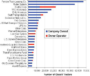
FIGURE 2-1 The 25 largest private and for-hire fleets. SOURCE: ATA (2007b). Used by permission of Transport Topics Publishing Group. Copyright 2009. American Trucking Associations, Inc.
5-year period (2004-2008), sales were down 30 percent for most classes, with only Class 5 showing a marginal increase of 6 percent (see Table 2-6). The Ward’s data on vehicle classes and manufacturers (Table 2-7) show:
-
Profound cycling of sales volumes, especially in higher weight classes.
-
Though still down, sales between the dominant providers, Ford and General Motors, shifted significantly as the GM share went from 2 percent (2004) to 37 percent (2008). Sales were down 27 percent over the period.
-
Classes 4 through 7 did not see significant shifts among the manufacturers—Ford, GM, International, Freight-liner, Hino, and Sterling. Diesel emission requirements and general economic unknowns both contributed to a nearly 40 percent decline in sales over the 5-year period.
-
Major manufacturers for Class 8 vehicles have not varied over the past 5 years with one exception—the case of Freightliner—whose market share has declined 5 percent since 2004.
As with vehicle sales, sales of engines manufactured for medium- and heavy-duty trucks declined from 764,000 units in 2004 to 557,000 in 2008 (Table 2-8).
The Class 8 vehicle and engine volumes illustrate profound fluctuations due to both a 2006 pre-buy to avoid cost increases and unknown reliability of 2007 emission controls, followed by the current U.S. recession.
INDUSTRY STRUCTURE
Chapter 1, among other things, reviews the economic power of the great industry built on heavy-duty vehicles and their users. Each year it accounts for billions of dollars in national income and millions of jobs: design engineers, drivers, manufacturing and maintenance technicians, materials handlers, and vehicle sales.
Unlike the makers of light-duty vehicles, which are dominated by a few very large companies (General Motors, Ford, and Toyota), manufacturers of trucks and buses are extremely varied in scale and depend on a web of suppliers, subcontractors, and service industries of all sizes and shapes. Even the largest builders of Class 8 trucks—Daimler, Navistar, PACCAR, and Volvo—each sell 18,000 to 80,000 units annually, and their relative market shares shift. For many medium-duty trucks, the manufacturer of record is essentially a body or equipment builder. The chassis and power train come from one of the major vehicle original equipment manufacturers (OEMs), but the body builder creates the final vehicle configuration. This approach is common for vehicles such as concrete mixers, school buses, utility trucks, and delivery trucks. In many cases the manufacturer of record has limited engineering resources and also limited influence over the fuel consumption of the vehicle. Even major vehicle OEMs sometimes buy components such as the engine, transmission, and axles, all of which have a significant impact on fuel consumption. Tractors and trailers are never built by the same company, and they are often not owned by the same company in actual operation. Even though the tractor-trailer truck’s
TABLE 2-2 Product Ranges of U.S. Heavy-Duty Vehicle Manufacturers
|
|
|
SOURCE: M.J. Bradley &Associates (2009). |
fuel consumption is determined by features of both the tractor and the trailer, no single company is responsible for the development of the complete vehicle. This industry structure will complicate any effort to regulate fuel consumption.
Engine manufacturers are also quite numerous. At least a dozen are contenders, according to Table 2-8, and are highly competitive. The same highly competitive situation is true of the commercial users of vehicles. At one end the highway is home for the truly independent operator, the long-distance trucker. At the other end are large fleets with thousands of trucks supported by sophisticated logistics and maintenance systems.
METRICS TO DETERMINE THE FUEL EFFICIENCY OF VEHICLES
Fuel Economy versus Fuel Consumption
In the wake of the 1973 oil crisis and energy security issues, Congress passed the Energy Policy and Conservation Act (P.L. 94-163) in 1975 as a means of reducing the country’s dependence on imported oil. The Act established the Corporate Average Fuel Economy (CAFE) program, which required automobile manufacturers to increase the average fuel economy of vehicles sold in the United States to a standard of 27.5 miles per gallon (mpg) for passenger cars. It also allowed the U.S. Department of Transportation (DOT) to set appropriate standards for light trucks. The standards are administered in DOT by the NHTSA on the basis of
TABLE 2-3 Top 10 Commercial Fleets in North America
|
Rank |
Company Name and Location |
Type of Business |
Total Trucks, 2009 |
Fuel Types |
Maintenance Services |
|
1 |
UPS Inc. Atlanta |
Package service |
93,552 |
Gas, diesel, CNG, hybrid electric, LNG, electric |
PM |
|
2 |
FedEx Memphis, Tenn. |
Package service |
65,000 |
Gas, diesel, hybrid electric |
PM, EO, HD, CM, EU |
|
3 |
Quanta Services Houston |
Utility construction |
24,000 |
Diesel |
PM |
|
4 |
Waste Management Houston |
Waste services |
22,000 |
Diesel, natural gas, hybrid electric |
PM, HD, EU |
|
5 |
Republic Services Phoenix |
Waste services |
21,399 |
Diesel, gas, biodiesel, natural gas, hybrid electric |
PM, EO, HD |
|
6 |
PepsiCo/Frito-Lay Purchase, N.Y. |
Food and beverage |
19,424 |
Gas, diesel, hybrid electric |
PM |
|
7 |
ServiceMaster Co. |
Home and business services |
15,706 |
Gas |
PM |
|
8 |
Aramark Philadelphia |
Uniform services and food and beverage |
10,968 |
Gas, diesel |
PM, EO, EU |
|
9 |
Cintas Corp. Cincinnati |
Uniform and business services |
9,500 |
Gas, diesel |
PM, EO |
|
10 |
Coca-Cola Enterprises |
Beverage bottler |
9,500 |
Diesel, gasoline, biodiesel, hybrid electric, electric |
PM, HD, CM |
|
SOURCE: ATA (2009), p. 16. |
|||||
TABLE 2-4 Top 10 Transit Bus Fleets in the United States and Canada
|
|
|
SOURCE: Courtesy of Metro Magazine (2009), p. 14. |
TABLE 2-5 Top 10 Motor Coach Operators, 2008, United States and Canada
|
|
|
SOURCE: Metro Magazine (2009), p. 24. |
TABLE 2-6 Medium- and Heavy-Duty-Vehicle Sales by Calendar Year
|
Vehicle Class |
Calendar Year |
Percent Change, 2004-2008 |
||||
|
2004 |
2005 |
2006 |
2007 |
2008 |
||
|
Class 3 |
136,229 |
146,809 |
115,140 |
156,610 |
99,692 |
−27 |
|
Class 4 |
36,203 |
36,812 |
31,471 |
35,293 |
21,420 |
−41 |
|
Class 5 |
26,058 |
37,359 |
33,757 |
34,478 |
27,558 |
6 |
|
Class 6 |
67,252 |
55,666 |
68,069 |
46,158 |
27,977 |
−58 |
|
Class 7 |
61,918 |
71,305 |
78,754 |
54,761 |
44,943 |
−27 |
|
Class 8 |
194,827 |
253,840 |
274,480 |
137,016 |
127,880 |
−34 |
|
TOTAL Sales |
522,487 |
601,791 |
601,671 |
464,316 |
349,470 |
−33 |
|
SOURCE: DOE/EERE (2009), p. 20, based on Ward’s Motor Vehicle Facts and Figures, available at http://www.wardsauto.com/about/factsfigures. |
||||||
U.S. Environmental Protection Agency (EPA) city-highway dynamometer test procedures.1
The terms fuel economy and fuel consumption are both used to show the efficiency of how fuel is used in vehicles. These terms need to be defined.
-
Fuel economy is a measure of how far a vehicle will go with a gallon of fuel and is expressed in miles per gallon (mpg). This is the term used by consumers, manufacturers, and regulators to communicate with the public in North America.
-
Fuel consumption is the inverse measure—the amount of fuel consumed in driving a given distance—and is measured in units such as gallons per 100 miles or liters per kilometer. Fuel consumption is a fundamental engineering measure and is useful because it is related directly to the goal of decreasing the amount of fuel required to travel a given distance.
TABLE 2-7 Truck Sales, by Manufacturer, 2004-2008
|
|
Calendar Year |
||||
|
2004 |
2005 |
2006 |
2007 |
2008 |
|
|
Class 3 |
|
|
|
|
|
|
Chrysler |
29,859 |
35,038 |
36,057 |
46,553 |
29,638 |
|
Ford |
68,615 |
122,903 |
105,955 |
81,155 |
60,139 |
|
Freightlinera |
270 |
14 |
0 |
0 |
0 |
|
General Motors |
2,471 |
2,788 |
2,578 |
33,507 |
41,559 |
|
International |
0 |
0 |
0 |
0 |
609 |
|
Isuzu |
4,992 |
5,167 |
4,929 |
4,350 |
2568 |
|
Mitsubishi-Fuso |
720 |
670 |
93 |
52 |
202 |
|
Nissan Diesel |
352 |
276 |
232 |
279 |
112 |
|
Sterling |
0 |
0 |
0 |
0 |
12 |
|
Total |
107,279 |
166,856 |
149,844 |
165,896 |
134,839 |
|
Classes 4-7 |
|
|
|
|
|
|
Chrysler |
0 |
0 |
0 |
588 |
5,386 |
|
Ford |
60,538 |
61,358 |
69,070 |
70,836 |
46,454 |
|
Freightlinera |
51,814 |
51,639 |
51,357 |
42,061 |
30,809 |
|
General Motors |
34,351 |
45,144 |
41,340 |
34,164 |
24,828 |
|
Hino |
2,387 |
4,290 |
6,203 |
5,448 |
4,917 |
|
Navistar/International |
52,278 |
54,895 |
61,814 |
40,268 |
35,022 |
|
Isuzu |
10,715 |
10,620 |
10,822 |
9,639 |
6,157 |
|
Kenworth |
5,020 |
3,874 |
5040 |
4,239 |
3,710 |
|
Mack |
21 |
0 |
0 |
0 |
0 |
|
Mitsubishi-Fuso |
4,384 |
4,842 |
5,967 |
5,218 |
2,136 |
|
Nissan |
0 |
0 |
0 |
0 |
0 |
|
Nissan Diesel |
2,453 |
2,382 |
2,551 |
2,080 |
1,273 |
|
Peterbilt |
4,495 |
4,739 |
6,307 |
5009 |
3,792 |
|
Sterling |
0 |
0 |
102 |
578 |
467 |
|
Total |
228,456 |
243,783 |
260,573 |
220,128 |
164,951 |
|
Class 8 |
|
|
|
|
|
|
Freightlinera |
73,731 |
94,900 |
98,603 |
51,706 |
42,639 |
|
Navistar/International |
38,242 |
46,093 |
53,373 |
29,675 |
32,399 |
|
Kenworth |
23,294 |
27,153 |
33,091 |
19,299 |
15,855 |
|
Mack |
20,670 |
27,303 |
29,524 |
13,438 |
11,794 |
|
Peterbilt |
26,145 |
30,274 |
37,322 |
19,948 |
17,613 |
|
Volvo Truck |
20,323 |
26,446 |
30,716 |
16,064 |
13,061 |
|
Other |
792 |
623 |
1,379 |
835 |
112 |
|
Total |
203,197 |
252,792 |
284,008 |
150,965 |
133,473 |
|
Grand Total |
538,932 |
663,431 |
694,425 |
536,989 |
433,263 |
|
aFreightliner/Western Star/Sterling(domestic). SOURCE: DOE/EERE (2009), pp. 21-22, based on Ward’s Motor Vehicle Facts and Figures, available at http://www.wardsauto.com/about/factsfigures. |
|||||
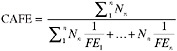
The CAFE for light-duty vehicles is calculated from fuel consumption data using a “harmonic average.”2 The harmonic average in the CAFE standards is determined as the sales weighted average of the fuel consumption for the Urban and Highway schedules, converted into fuel economy. The average is calculated using the fuel consumption of individual vehicles times the number of vehicles sold of each model, summed over the whole fleet and divided by the total fleet.
TABLE 2-8 Engines Manufactured for Class 2b Through Class 8 Trucks, 2004-2008
|
|
2004 |
2005 |
2006 |
2007 |
2008 |
|
Engines Manufactured for Heavy-Duty Trucks |
|||||
|
Cummins |
64,630 |
79,100 |
91,317 |
65,228 |
75,307 |
|
Detroit Diesel |
48,060 |
61,074 |
63,809 |
29,506 |
35,174 |
|
Caterpillar |
74,224 |
86,806 |
97,544 |
33,232 |
20,099 |
|
Mack |
25,158 |
36,211 |
36,198 |
18,544 |
16,794 |
|
Mercedes Benz |
17,178 |
24,414 |
24,584 |
17,048 |
10,925 |
|
Volvo |
12,567 |
19,298 |
23,455 |
9,850 |
8,822 |
|
Navistar |
0 |
0 |
0 |
4 |
927 |
|
PACCAR |
0 |
0 |
0 |
52 |
20 |
|
Total |
241,817 |
306,913 |
336,907 |
173,464 |
168,068 |
|
Engines Manufactured for Medium-Duty Trucks |
|||||
|
Navistar |
373,842 |
382,143 |
357,470 |
335,046 |
264,317 |
|
GM |
74,328 |
77,056 |
83,355 |
87,749 |
72,729 |
|
Cummins |
14,900 |
15,162 |
16,400 |
20,615 |
27,664 |
|
Mercedes Benz |
16,075 |
20,038 |
27,155 |
19,330 |
9,066 |
|
Caterpillar |
42,535 |
42,350 |
45,069 |
14,693 |
6,269 |
|
PACCAR |
0 |
0 |
0 |
9,020 |
5,694 |
|
Hino |
671 |
5,001 |
7,489 |
6,230 |
3,062 |
|
Detroit Diesel |
0 |
958 |
8 |
0 |
0 |
|
Total |
522,351 |
542,708 |
536,946 |
492,683 |
388,801 |
|
Engines Manufactured for Medium- and Heavy-Duty Trucks |
|||||
|
Navistar |
373,842 |
382,143 |
357,470 |
335,050 |
265,244 |
|
Cummins |
79,530 |
94,262 |
107,717 |
85,843 |
102,971 |
|
GM |
74,328 |
77,056 |
83,355 |
87,749 |
72,729 |
|
Detroit Diesel |
48,060 |
62,032 |
63,817 |
29,506 |
35,174 |
|
Caterpillar |
116,759 |
129,156 |
142,613 |
47,295 |
26,368 |
|
Mercedes Benz |
33,253 |
44,452 |
51,739 |
36,378 |
19,991 |
|
Mack |
25,158 |
36,221 |
36,198 |
18,544 |
16,794 |
|
Volvo |
12,567 |
19,298 |
23,455 |
9,850 |
8,822 |
|
PACCAR |
0 |
0 |
0 |
9,072 |
5,714 |
|
Hino |
671 |
5,001 |
7,489 |
6,230 |
3,062 |
|
Total |
764,168 |
849,621 |
873,853 |
666,147 |
556,869 |
Because fuel economy and fuel consumption are reciprocal, each of the two metrics can be computed in a straightforward manner if the other is known. In mathematical terms, if fuel economy is X and fuel consumption is Y, their relationship is expressed by XY = 1. This relationship is not linear, as illustrated by Figure 2-2. In this figure, fuel consumption is shown in units of gallons/100 miles, and fuel economy is shown in units of miles/gallon. The figure also shows that a given percentage improvement in fuel economy saves less and less fuel as the baseline fuel economy increases. Each bar represents an increase in fuel economy by 100 percent, which corresponds to a decrease in fuel consumption by 50 percent. The data on the graph show the resulting decrease in fuel consumption per 100 miles and the total fuel saved in driving 10,000 miles. The dramatic decrease in the impact of increasing fuel economy by 100 percent for a high fuel economy vehicle is most visible in the case of increasing the fuel economy from 40 to 80 mpg, where the total fuel saved in driving 10,000 miles is only 125 gallons, compared to
 where Nn = number of vehicles in class n, FEn = fuel economy of class n vehicles and n = number of separate classes of vehicles.
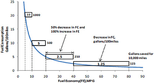
FIGURE 2-2 Fuel consumption (FC) versus fuel economy (FE), showing the effect of a 50 percent decrease in FC and a 100 percent increase in FE for various values of FE, including fuel saved over 10,000 miles. Results are based on Eq 2-1.
1,000 gallons for a change from 5 to 10 mpg. Appendix E discusses further implications of the relationship between fuel consumption and fuel economy for various fuel economy values.
Fuel consumption difference is also the metric that determines the yearly fuel savings in going from a given fuel economy vehicle to a higher fuel economy vehicle:
(Eq. 2.1)
where FC1 = fuel consumption of existing vehicle, gallons/100 miles, and FC2 = fuel consumption of new vehicle, gallons/100 miles.
The amount of fuel saved for a light-duty vehicle in going from 14 to 16 mpg for 12,000 miles per year is 107 gallons. This savings is the same as a change in fuel economy for another vehicle in going from 35 to 50.8 mpg. The amount of fuel saved for a heavy-duty truck in going from 6 to 7 mpg for 12,000 miles per year is 286 gallons, which is more than double the fuel savings of the light-duty vehicle examples. Once the average long-haul tractor vehicle miles traveled of 120,000 miles per year is considered, the fuel savings for an increase from 6 to 7 mpg is 2,857 gallons. This is 26.7 times more fuel savings than for the two car examples. The fuel savings achieved by a heavy truck going from 6 to 7 mpg is also the same as a change in fuel economy for a medium-duty vehicle in going from 10 to 13.1 miles per gallon, assuming identical driving distance. In practice, medium-duty trucks tend to drive fewer miles, so a higher fuel economy improvement would be required to save an equal amount of fuel. Equation 2.1 and these examples again show how important the use of fuel consumption metric is to judge yearly fuel savings.
Because of the nonlinear relationship in Figure 2-2, consumers of light-duty vehicles have been shown to have difficulty using fuel economy as a measure of fuel efficiency in judging the benefits of replacing the most inefficient vehicles. Larrick and Soll (2008) conducted three experiments to test whether people reason in a linear but incorrect manner about fuel economy. These experimental studies demonstrated a systemic misunderstanding of fuel economy as a measure of fuel efficiency. Using linear reasoning about fuel economy leads people to undervalue small improvements (1 to 4 mpg) in lower-fuel-economy (15 to 30 mpg range) light-duty vehicles, despite the fact that there are large decreases in fuel consumption in this range, as shown in Figure 2-2. This problem worsens when fuel economy numbers typical of trucks and busses are considered (3 to 12 mpg).
Clearly, fuel economy is not a good metric for judging the fuel efficiency of a vehicle. The CAFE standards for light-duty vehicles are expressed in terms of fuel economy, although fuel consumption of individual vehicles is used in the calculation of the sales weighted harmonic average fuel economy. To be consistent throughout this report, fuel consumption is used as the metric. It is the fundamental measure of fuel efficiency both in the regulations and for judging fuel savings by consumers and truck operators. Figure 2-3 was derived from Figure 2-2 to show how percent of fuel
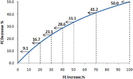
FIGURE 2-3 Percentage fuel consumption (FC) decrease versus percentage fuel economy (FE) increase.
consumption decrease is related to percent increase of fuel economy. The curve in Figure 2-3 is independent of the value of fuel economy. Where fuel economy increase data have been used from the literature, or from fleets, manufacturers of vehicles, and component suppliers, this figure or an equation3 has been used to convert the data to a fuel consumption decrease in percent.
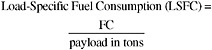
Load-Specific Fuel Consumption
Medium- and heavy-duty vehicles are unlike light-duty vehicles in that they are clearly designed to carry loads in an efficient and timely manner. In the EPA light-duty vehicle fuel economy tests, the only load in the vehicle during the test is one 150-lb person as the driver. This is the typical way these vehicles operate, although different light-duty vehicles have the capacity to carry additional passengers and cargo, depending on their size. Delivering the driver and passengers to a destination can be considered the primary purpose of light-duty vehicles. On the other hand, the primary purpose of most medium- and heavy-duty vehicles is to deliver freight or passengers (the payload). A simple way to reduce the fuel consumption of a truck is to leave the cargo on the loading dock. This approach, however, ignores the purpose of these vehicles. In view of these facts, the way to represent an appropriate attribute-based fuel consumption metric is to normalize the fuel consumption to the payload that the vehicle hauls. This is represented by the following equation:
(Eq. 2.2)
where FC = fuel consumption on a given cycle, gallons/100 miles. The literature also shows data represented by the following equation:
(Eq. 2.3)
(Eq. 2.4)
where FE = fuel economy on a given cycle, miles/gallons.
It is important to note that the payload of a vehicle significantly affects the fuel economy (FE), fuel consumption (FC), and LSFC as shown in Figures 2-4, 2-5, and 2-6. These results are from simulations for a line-haul vehicle and an urban delivery vehicle in operations based on real-world routes recorded by Cummins. Table 2-9 shows a few of the variables used for the simulations in Figures 2-4 through 2-6. Note that adding payload to a vehicle increases fuel consumption, but the higher payload actually improves
|
3 |
If FEf = (FE2 − FE1)/FE1 and FCf = (FC1 − FC2)/FC2 where FE1 and FC1 = FE and FC for vehicle baseline and FE2 and FC2 = FE and FC for vehicles with advanced technology, then, FCf = FEf /(FEf + 1) where FEf = fractional change in fuel economy and FCf = fractional change in fuel consumption. This equation can be used for any change in FE or FC to calculate the values shown in Figure 2-2. Also, FEf = FCf /(1 − FCf) and % FC = 100 FCf, % FE = 100 FEf. |
FIGURE 2-6 Load-specific fuel consumption versus payload. SOURCE: Jeffrey Seger, Cummins, Inc., personal communication, June 6, 2009.
the efficiency of the vehicle (in terms of LSFC). Failure to understand this counterintuitive fact can lead to regulations with severe unintended consequences.
Payload is an important variable to input for either a vehicle computer simulation or an experimental test for determining a vehicle’s fuel consumption. The duty cycle that the vehicle operates on is also important. Another important variable is average vehicle speed. It is important that any regulation use an average payload based on national data representative of the class and duty cycle of the vehicle. Appendix E gives national data for the average payload of various classes of vehicles. Buses could use the average number of typical passengers times an average weight (150 lb as used in light-duty standards) plus some average baggage weight for each passenger (perhaps 25 to 35 lb).
NHTSA would use the data in Appendix E or other payload data to arrive at a simple specific average or typical payload for each class and for each separate vehicle application within a class e.g. tractor trailer, box truck, bucket truck, refuse truck, transit bus, motor coach, etc, for carrying out vehicle certification testing/simulation. For example, this payload would be at a given point in Figures 2-4 to 2-6.
If the payload for a line-haul truck was 20 tons, LSFC would be about 0.9 gallons/ton-100 miles. This might be the example for a typical grossed-out (at maximum cargo weight) vehicle. If the payload was 6 tons for the example of an urban delivery cubed-out (at maximum cargo volume) vehicle, the LSFC would be about 1.3 gallons/ton-100 miles. Now, how can the LSFC be reduced? Since the payload for the test/simulation for a given vehicle is fixed, the engine and vehicle technology discussed in Chapters 4 and 5 can be used to reduce FC, increase FE and reduce LSFC. Weight reduction of the vehicle can also be used to reduce LSFC at the specified payload which would allow full-load payload to be increased for the grossed-out vehicle. In the cubed-out vehicle example, the payload volume can be increased, new technology added, and weight reduced to reduce FC, increase FE, and reduce LSFC. This would allow the cubed-out vehicle to carry more low-density cargo.
TABLE 2-9 Vehicle, Engine, and Cycle Variables
|
|
Line Haul |
Urban Delivery |
|
Vehicle weight empty (lb) |
33,500 |
7,500 |
|
Engine power (hp) |
450 |
245 |
|
Length of route (miles) |
65.66 |
100 |
|
Average vehicle speed (mph) |
60.5 |
19.2 |
|
Payload (lb) |
0-55,000 |
0-24,000 |
|
SOURCE: Jeffrey Seger, Cummins, Inc., personal communication, June 6, 2009. |
||
Using LSFC in these two examples provides an incentive for industry to reduce FC and LSFC. The key to this approach is a specified typical payload: payload cannot be changed to improve LSFC. The other important point is that this approach is not a full-payload test/simulation unless the vehicle always operates at this load. Clearly, because the levels of FC and LSFC from Figures 2-5 and 2-6 vary widely depending on the type of vehicle and payload, there will be a need for different standards for different vehicle classes and corporate fleet averaging.
Further, it is important that any standard for fuel efficiency be based on LSFC, since it focuses on reducing the fuel consumed by medium-and heavy-duty vehicles sold in the United States, when operating on cycles representative of their work-duty cycles. LSFC can be used directly times the number of vehicles and averaged over the fleet if NHTSA desires to use a fleet average standard for vehicles of a given class that operate in a similar manner. Payload is
an important variable that affects FC and LSFC; therefore, any reported values or labels should state FC = gallon/100 miles and LSFC = gallons/ton-100 miles at specific tons of payload.
TRUCK TRACTIVE FORCES AND ENERGY INVENTORY
It is instructive to review the fundamental vehicle attributes that account for fuel consumption before examining the technologies that could reduce fuel consumption.
Road Load
The force or power required to propel a vehicle at any moment in time is customarily presented as a “road load equation.” For the case of force, the equation has four terms to describe tire rolling resistance, aerodynamic drag, acceleration, and grade effects:
where mg is vehicle weight, Crr is tire rolling resistance, A is the frontal area, Cd is a drag coefficient based on the frontal area, ρa is the air density, V is the vehicle velocity, m is vehicle mass, t is time, and sin(θ) is the road gradient (uphill positive). Neither CD nor Crr need be constant with respect to speed, and the term CDA should not be split without careful thought.
For road load power, the force equation is merely multiplied by the velocity:
In conventional vehicles the road load power is supplied by an engine, via a transmission and one or more drive axles characterized by an efficiency (η).The engine may also supply power for auxiliary loads (Paux), including cooling fan loads, so that a simple engine power demand (PE) model is given by:
The force FRL may become negative while the vehicle is decelerating or traveling on a sufficiently steep downgrade, with “negative” power being absorbed through engine braking or friction brakes. For hybrid-drive vehicles, some of the “negative” power may be absorbed and stored for use in future propulsion of the vehicle. Since hybrid vehicles have at least two sources of power during part of their duty cycle, the engine power demand model must be adjusted to account for the flow of power to or from other sources during operation.
A specific engine type may be used in a variety of vehicle applications and may be coupled to the wheels via a variety of drivetrains, so that the in-use engpe the average power demand, fuel consumption, and energy required to travel a specific distance vary substantially with the vehicle activity, or duty cycle. The average engine efficiency will also be impacted by the duty cycle, as is the contribution of each major element of the road load equation (aerodynamics, weight, tires) to the overall vehicle fuel consumption. Figure 2-7 illustrates how the extremes of duty cycles can create a wide range of impacts of the specific vehicle attributes to the overall vehicle fuel consumption.
When either engines or vehicles are to be certified for efficiency or emissions standards, it is necessary to establish test cycles to challenge the vehicle or engine, but it has historically been accepted in regulations that these tests cannot hope to represent every in-use behavior. This is discussed further later in this chapter and in Chapter 3.
TEST PROTOCOLS
Fuel consumption may be measured directly from a vehicle on the road, a test track, or a chassis dynamometer. It is important to distinguish between comparative testing, where fuel consumption values used by two trucks of different technology are compared, and absolute testing, where fuel consumption is measured using a standardized procedure so that the results may be compared with results from tests conducted at different times or in different locations. If onroad measurement is conducted over a long distance or long period of time, the resulting average fuel consumption values may be compared fairly with those from another vehicle operated over a sufficiently similar route with sufficiently similar operating conditions. The purpose of a test track is to provide sufficiently repeatable conditions and vehicle activity that a comparison between the performances of two vehicles is possible with a reduced distance or time of operation relative to less controlled on-road tests.
A chassis dynamometer simulates road load on a vehicle while the vehicle drive wheels operate on rollers rather than a road surface. This provides a high degree of repeatability in testing but requires that the effective vehicle mass is known and that road load constants are available. These constants are associated with the rolling resistance Crr and CdA but cannot be computed directly from them because there is an offset associated with drive train losses. It is customary, especially for passenger cars, to perform an on-road coast-down test of the vehicle to obtain the road load constants, discussed in subsequent sections.4
Both on-road and chassis dynamometer measurement methods are described in EPA SmartWay documents.
The Recommended Practices of the Society of Automotive Engineers (SAE) present details of road testing and of chassis dynamometer methods to determine hybrid and conventional vehicle fuel economy.5
Fuel-use data from on-road tests or chassis dynamom-
FIGURE 2-7 Energy “loss” range of vehicle attributes as impacted by duty cycle, on a level road.
eter tests may be used indirectly to calibrate whole-vehicle models where Crr and CDA are not known directly or independently. The model may be used, in turn, to predict fuel consumption on unseen cycles.
On-Road Testing
Physical Testing—Powered: SAE J1321 Fuel Consumption Test Procedure, Type II
This procedure measures on-road fuel consumption utilizing a similarly equipped, unchanging control vehicle operated in tandem with a test vehicle to provide reference fuel consumption data. This procedure has become the de facto test for both carrier and manufacturer fuel economy evaluations, largely due to its ability to use real-world vehicles and routes.
The specification requires both careful control of potential operational variables and numerous replications to validate the difference statistics. The procedure is claimed to provide precision within ±1 percent. The committee’s analysis suggests that the current precision, acquired from three T/C6 ratios within a 2 percent range, results in a standard deviation in the range of 0.9 to 1.1 percent. So, the precision of the SAE J1321 result is more nearly ±2 percent for 95 percent confidence and ±3 percent for 99 percent confidence.
This full-truck system validation includes aerodynamic losses and produces results in percent of reduction in fuel consumption over whatever road type is selected, e.g., from a track or to a specific carrier route. When conducted by expert third-party labs, evaluation of a base case plus three variables can cost $33,000.
For evaluation of aerodynamic systems alone, it may be helpful to use unladed trucks. This process decreases the total fuel consumed so that the incremental consumption of the test truck is larger than in the laded condition. Unfortunately, the procedure has no systematic process for accounting for side winds (yaw conditions), which is a clear and significant aerodynamic shortcoming.
EPA modified the SAE J1321 test procedure (TP) to require use of a test track environment, and each test segment incurs only one acceleration and deceleration. It measures fuel consumption and requires that average speed be controlled to 55 to 62 mph preferred, 65 mph maximum (EPA, 2009).
Coast Down: SAE J1263 Test Procedure
Coast-down testing, as mentioned earlier, is performed to define the rolling resistance and characteristic aerodynamic drag of a vehicle as inputs for a chassis dynamometer load setting. The coast-down process7 must be well regulated and avoid uncharacteristic wind drag or gradients and will be dependent on vehicle mass and the nature of the road surface.8
This procedure is now used infrequently as the other test procedures have gained increased use due to their more acceptable precisions. Coast-down tests are complicated by prevailing winds that reduce the overall precision of the procedure.
Physical Testing—Wind Tunnel: SAE J1252 Test Procedure
The SAE J1252 test procedure measures aerodynamic drag force directly, from which the Cd is calculated. A wind tunnel is the only accurate method to measure the yaw force and thereby the Cd in yaw. This TP also provides for the calculation of a wind average drag coefficient. The drag curve for a tractor with a 45-ft trailer in Figure 5-7 would have a wind average Cd about 15 percent higher than the 0° Cd. That fact begs for a wind average measurement, particularly since certain devices are better at reducing drag in yaw than at 0°. The gap region and trailer (rear) base are particularly sensitive to oblique wind conditions.
After construction of a base tractor and trailer models, evaluation of three variables can cost $7,000, in addition to the base models’ fabrication.
The National Aeronautics and Space Administration has developed a correlation between complete truck Cd and fuel consumption.
Computational Fluid Dynamics
Over the past 6 years, computational fluid dynamics (CFD) codes have found increased application to the flow and drag conditions in truck aerodynamics management, encouraged by the DOE. CFD uses numerical methods and algorithms to analyze and solve problems that involve fluid flows. Computers are used to perform the millions of calculations required to simulate the interaction of fluids and gases with the complex surfaces used in engineering. The computer codes/procedures often embody unique individualities of their various developers, and no single practice has emerged as a standard.
Manufacturers are increasingly using this tool to provide details of aero effects helpful to differentiate multiple design features even before building models for wind tunnel evaluation. They have found CFD complements wind tunnel results, which can directly provide Cd results (TMA, 2007, pp. 7, 20). Another recent study concluded that through the example of the Jaguar XF program a combination of (CFD) simulation and relatively simple full-scale wind tunnel testing can deliver competitive aerodynamic performance (Gaylard, 2009).
Chassis Dynamometers
Chassis dynamometers must mimic vehicle inertia and road load for transient cycle evaluations. Simpler dynamometers developed to measure only vehicle power output are unsuited for general fuel consumption measurement. In most cases both inertia and road load forces are applied between the wheel and the roller, but in other cases the drive hubs themselves may be connected mechanically to a dynamometer system. The inertia effect may be applied by either using flywheels or applying torque generated by a substantial electric motor/generator and controlled to apply the torque in proportion to vehicle acceleration and deceleration. Road load may be applied by the same substantial electric machine, or by a smaller electric motor/generator, eddy current power absorber or hydraulic power absorber used in conjunction with flywheels. Flywheels offer the advantage of mimicking inertia faithfully at very low speeds, while systems with a large electric motor/generator may also be used to mimic gradients.
Light-duty vehicle dynamometers for U.S. emissions certification use are well described and employ a single 4-ft-diameter roll under the drive axle. Use of these dynamometers is closely prescribed in the Code of Federal Regulations. Other common light-duty designs use four rolls for inspection and maintenance implementation and for garage-grade testing. Heavy-duty units are few in number and vary in design.
A dynamometer test sequence consists of a coast-down (or equivalent, explained in previous section) method to set road load for a given inertial weight, followed by exercising the vehicle through a cycle by a human driver instructed by a video screen speed-time graph. Fuel used may be measured using emissions measurement equipment to determine carbon dioxide and fuel analysis to determine carbon content. Alternatively, fuel mass used may be determined directly by a scale or measured volumetrically. Fuel flow rate is also broadcast by most modern engines but is insufficiently accurate for fuel consumption determination.
Validation of Test Results
The SAE has tasked its Truck and Bus Aerodynamic and Fuel Economy Committee to bring the various current SAE procedures and practices into the needs of the 21st century, reflective of prevailing engineering and scientific data analysis to facilitate robust validation. An early assessment of the SAE committee is that “uncertainty analysis” must play a key role in achieving the overarching goal of providing unified industry standards for validating fuel consumption of heavy trucks and buses, including their aerodynamic properties. Indeed, this study will also assess if new procedures are required. This SAE committee is represented by wide participation across industry and academia.
The committee believes that this SAE committee should be specifically requested to provide a summary and rationale for the completion of Table 2-10. This table considers the
TABLE 2-10 Validation, Accuracy, and Precision
|
Parameter |
SAE J1321 |
EPA-Mod J1321 |
Coast Down |
Wind Tunnel |
CFD |
Full-Truck Computer Simulation |
|
Accuracy |
% |
% |
% |
% |
% |
% |
|
Precision |
% |
% |
% |
% |
% |
% |
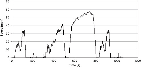
FIGURE 2-8 The Heavy-Duty Urban Dynamometer Driving Schedule. SOURCE: Clark (2003). Reprinted with permission from SAE. © 2003 SAE International.
adequacy of influencing parameter control pertinent to each validation process. Variables of concern include vehicle speed, wind speed and direction (yaw), temperature, humidity, wind tunnel variables, geometry modeling, flow modeling, fuel, lubricants, and driver.
TEST-CYCLE DEVELOPMENT AND CHARACTERISTICS
Development of Test Cycles
In characterizing the fuel efficiency of a whole vehicle (or of a chassis or mule created to mimic a whole vehicle) against a standard, it is essential to exercise the vehicle through a prescribed speed-time sequence that reasonably reflects actual use. Such has been the case for passenger vehicles. For emissions regulations for heavy-duty vehicles, the representative test cycles are applied to only the engine on an engine dynamometer. However, many nonregulatory test cycles have been developed and documented for heavy vehicles for a variety of purposes. The EPA’s Heavy-Duty Urban Dynamometer Driving Schedule (UDDS) is set by regulation (40 CFR 86, App. I) as a vehicle conditioning cycle. The UDDS (Figure 2-8) was created using Monte Carlo simulation with a statistical speed-acceleration basis, and it has origins similar to those of the heavy-duty engine certification test used for implementation of emissions standards for diesel engines. The UDDS includes “freeway” and “nonfreeway” activity.
Engineers typically assemble cycles in this way, by combining real-world truck activity data. An activity database may be created by logging speed from one or many trucks over a representative period of time. The log is then divided into “trips” or “microtrips,” either with idle activity separated or included with microtrips. A number of microtrips are then connected to form a cycle of desired length. Many such cycles are created from the database, and the cycle that is statistically most representative of the whole database, using metrics such as average speed and standard deviation of speed, is chosen as a representative cycle. Examples include the suite of “modes” of the Heavy Heavy-Duty Diesel Truck (HHDDT) schedule used in the E-55/59 California truck emissions inventory program. The idle, creep, transient, cruise, and high-speed cruise modes represent progressively higher average speeds of operation (Gautam et al., 2002; Clark et al., 2004). The creep and cruisecreep and cruise modes are shown in Figure 2-9. In a similar fashion, a Medium Heavy-Duty Schedule was also created (Clark et al., 2003).
Cycles have also been created to represent vocational truck and bus behavior. The National Renewable Energy Laboratory has proposed a refuse truck cycle for use in the EPA SmartWay program (EPA, 2009). The Hybrid Truck Users Forum Class 4 and Class 6 Parcel Delivery Cycles are also reported here. The “William H. Martin” cycle has been developed for refuse truck operation, which is acknowledged to vary widely in characteristics.
Transit bus fuel consumption has traditionally been established on test tracks.9 The SAE, in Recommended Practice J1376, provides a test procedure with three segments (Central Business District, Arterial, and Commuter) that mimic stop-and-go track testing for transit buses. These have been applied to bus testing on chassis dynamometers (Wang et al., 1994, 1995) and are “geometric” in nature. Figure 2-10 shows the Central Business District, which consists of idle, acceleration, cruise, and deceleration periods, with the acceleration and deceleration portions reflecting the abilities of a particular bus at the time of the cycle’s creation.
|
9 |
See “Bus Research and Testing Facility (Test Track)” at http://www.vss.psu.edu/BTRC/btrc_test_track.htm (accessed September 22, 2009). |
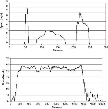
FIGURE 2-9 The creep (top) and cruise (bottom) modes of the HHDDT schedule. SOURCE: Clark (2003). Reprinted with permission from SAE. © 2003 SAE International.
Bus cycles developed from microtrips include the Manhattan and Orange County Transit Authority (OCTA) cycles10 (see Figure 2-11) and the Washington Metropolitan Area Transit Authority cycle (Wayne et al., 2008). Numerous additional bus and truck cycles receive attention on the website dieselnet.com and by Wayne et al. (2008) and Davies et al. (2005).
Application of a Cycle
On a chassis dynamometer, the vehicle speed provides for unambiguous wind drag and rolling resistance terms provided that the frontal area, drag coefficient, air density, vehicle mass, gravitational acceleration, and tire rolling resistance coefficient are known. The vehicle mass, acceleration, and deceleration derived from the speed plot provide the inertial term. Usually, no grade term is assumed, although limited research has been conducted on cycles incorporating grades (Walkowicz, 2006; Thompson et al., 2004). The dynamometer may be configured to mimic loads directly, or the dynamometer may be set to match a speed-time coast-down curve obtained from the vehicle during an on-road test.11
Cycle Characteristics
The average speed of a real-world cycle implies the level to which the cycle includes transient speed behavior. Very low speed cycles have high idle content, and idle content diminishes. In the same way, values such as “stops per unit distance,” average instantaneous acceleration or deceleration, and coefficient of variance of speed become smaller as average speed rises. Table 2-11 shows selected parameters from four truck cycles.
Consider a specific truck being operated at a defined weight. The fuel efficiency of that truck, in units of fuel consumed per unit distance, will vary substantially with respect
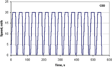
FIGURE 2-10 Central Business District segment of SAE Recommended Practice J1376.
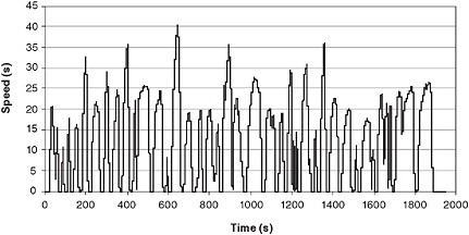
FIGURE 2-11 Orange County Transit Authority cycle derived from transit bus activity data. SOURCE: SAE.
TABLE 2-11 Characteristics of Selected Cycles
|
Parameter |
Filtered Creep Mode of HHDDT |
Filtered Transient Mode of HHDDT |
Filtered Cruise of HHDDT |
Test-D (UDDS) |
|
Duration (sec) |
253 |
668 |
2083 |
1063 |
|
Distance (miles) |
0.124 |
2.85 |
23.1 |
5.55 |
|
Average speed (mph) |
1.77 |
15.4 |
39.9 |
18.8 |
|
Stops/mile |
24.17 |
1.8 |
0.26 |
2.52 |
|
Maximum speed (mph) |
8.24 |
47.5 |
59.3 |
58 |
|
Maximum acceleration (mph/s) |
2.3 |
3 |
2.3 |
4.4 |
|
Maximum deceleration (mph/s) |
−2.53 |
−2.8 |
−2.5 |
−4.6 |
|
Total KE (mph-squared) |
3.66 |
207.6 |
1036 |
373.4 |
|
Percentage idle |
42.29 |
16.3 |
8 |
33.4 |
|
SOURCE: Data from CRC (2002). |
||||
to the vehicle activity or duty cycle (Graboski et al., 1998; Nine et al., 2000).
The effect of drive cycle is also well documented for light-duty vehicles and is known to affect emissions in addition to fuel economy (Nam, 2009; Wayne et al., 2008). It is essential to define the activity or cycle that the truck will follow before stating the associated fuel efficiency. The road load equation may be used to compute the power needed to propel a defined vehicle at steady speed over level terrain. The fuel consumed by the vehicle reflects this power requirement, but disproportionately more fuel is consumed at light loads for most conventional vehicles due to the inefficiency of an engine at light load conditions. The plot of fuel consumed (as l/100 km) against the steady speed is a curve that is concave upward. The fuel consumption tends to infinity at
idle (zero speed) because fuel is consumed with no distance gained. The curve has a minimum at some midspeed where aerodynamic drag forces are not yet excessive and the engine is at high efficiency, and the curve turns upward at high speed where aerodynamic forces start to dominate the energy required for propulsion. The minimum occurs at low speeds for vehicles with a high ratio of drag to rolling resistance. In this way the minimum occurs at low speeds for automobiles and at high speed for heavily loaded large trucks. Figure 2-12 shows the results of Argonne National Laboratory’s PSAT (Power Train Systems Analysis Toolkit) simulations for steady-state operation of two classes of heavy-duty vehicles, with a clear minimum in fuel consumption.
Vehicles in the real world do not operate at steady speed. For a given segment of activity, or for a cycle, it is therefore important to use the metric of average speed in discussing fuel use. Trucks operating at high average speed on freeways tend to be driven at a sustained, fairly steady speed, but trucks operating at lower speed in suburban or urban environments tend to vary their speed substantially, and urban activity is associated with frequent stops. A measure of speed variability is the standard deviation of speed (taken at one-second intervals) over a cycle. The standard deviation of speed does not vary linearly with the average speed. Figure 2-13 shows data for a number of cycles used in transit bus testing and shows a correlation between the standard deviation of speed and the average speed. This suggests that the average speed of a cycle conveys more information than the value of average speed itself: it also conveys the inherent transient nature of lower average speed operation. Figure 2-14 shows that the average speed also offers correlation with the percentage of time that a vehicle idles in the cycle and the number of times that the vehicle stops per mile of travel. Both idle operation and stop-start behavior are more common at low average
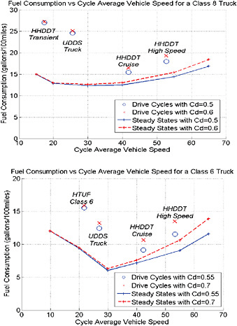
FIGURE 2-12 PSAT simulation results for steady-state operation and for selected transient test cycles for a Class 8 truck (top) and a Class 6 truck (bottom). The Class 6 truck modeled at 9,070 kg was based on a GMC C Series, and the Class 8 truck modeled at 29,931 kg was based on a Kenworth T660 with Cummins 14.9 L ISX. SOURCE: ANL (2009), Figures 26 and 28.
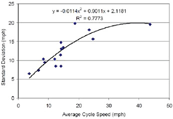
FIGURE 2-13 Standard deviation of speed changes (coefficient of variance rises) as the average speed drops for typical bus activity. SOURCE: Wayne et al. (2008). Reprinted with permission from the Transportation Research Forum.
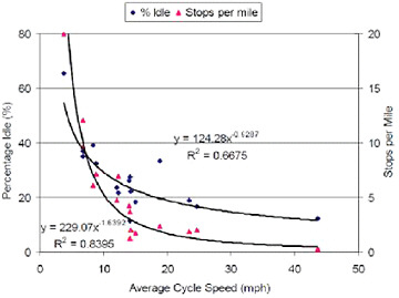
FIGURE 2-14 Percentage of time spent idling rises and there are more stops per unit distance as the average speed drops for typical bus activity. SOURCE: Wayne et al. (2008). Reprinted with permission from the Transportation Research Forum.
speed operation than on freeways. Freeways operating in choked condition will imply low average truck speeds, and the truck activity will more closely resemble urban activity than open freeway activity. Further evidence supporting the correlation between the nature of activity and the average speed of activity is provided elsewhere in a plot for data from automobiles.12
The effect of the increased transient behavior at low speeds is to raise the quantity of fuel consumed at low speeds. This is mainly due to the wasting of energy with service brakes and the associated need for propulsion energy during the next acceleration event. In addition, some power trains are less efficient under transient operation than under steady operation. If distance-specific fuel consumption is plotted against average speed, a curve is produced that is concave upward, with high values near zero speed, a minimum at midspeed, and rising values at very high speeds when aerodynamic forces start to dominate. The four cycles in Figure 2-12 also show the role that aerodynamic forces play in determining the speed at which the curve turns upward for typical Class
|
12 |
Available from California Air Resources Board, http://www.arb.ca.gov/msei/onroad/downloads/tsd/Speed_Correction_Factors.pdf. |
6 and Class 8 trucks. Curves of this kind have long been used in normalized form for emissions inventory models as “speed correction factors” to adjust distance-specific emissions when average speed deviates from the average speed of a reference cycle used to measure emissions (Frey and Zheng, 2002; Nam, 2009).
Real-world bus data to support the concept further are shown in Figure 2-15. Hybrid vehicles, which store braking energy for reuse during acceleration, and which may increase transient and light load power train efficiency, will primarily produce benefits at low speed. Figure 2-15 shows two best-fit curves for a 40-ft conventional (automatic transmission, diesel) transit bus and a hybrid (diesel) transit bus of similar size and weight. The curves are fitted to chassis dynamometer data taken using numerous transient cycles, each with a representative average speed. The fuel efficiency advantage of the hybrid bus at low operating speeds is evident.
Reporting Fuel Consumption from Different Cycles
The fuel efficiency of a truck is not readily characterized by a single number, but rather by a curve against average speed. Figures 2-14 and 2-15 suggest an approach that may be used to represent the fuel efficiency of a truck to an interested party. If varying operating weight is also considered a factor, fuel efficiency information forms a surface of values against the axes of average speed and operating weight. Creating curves or surfaces of this kind would require exhaustive chassis dynamometer measurements, but they may also be created using models that are calibrated with more limited chassis dynamometer data. Curves or surfaces would show that some technology has low-speed benefits and some has high-speed benefits and that some technology is more sensitive to payload than other technology.
Vehicle Simulation
As new power train and vehicle technologies appear, there will be an on-going challenge to make sure that the simulation tools provide an adequate representation of actual vehicle performance and fuel consumption. In this report, vehicle modeling and simulation will be used to assess the impact of current and future technologies on fuel consumption (see Appendixes G and H). While numerous modeling studies are available in the literature, the assumptions associated with the results are not always available. The committee decided to perform simulation studies using PSAT to analyze the impact of metric selection and assess the impact of current and future technologies. In addition, vehicle modeling will be assessed as part of the regulatory process.
In a world of growing competitiveness, the role of simulation in vehicle development is constantly increasing to allow engineers to bring new technologies to the market faster by reducing the need for hardware testing. Because of the number of possible advanced power train architectures and component technologies that can be employed, the development of the next generation of vehicles requires accurate, flexible simulation tools. Such tools are necessary to quickly narrow the technology focus to those configurations and components that are best able to reduce fuel consumption and performance.
Because models are a mathematical representation of physical components, different levels of fidelity will be used to represent different phenomena. As such, different approaches will be used to answer specific questions. At a high
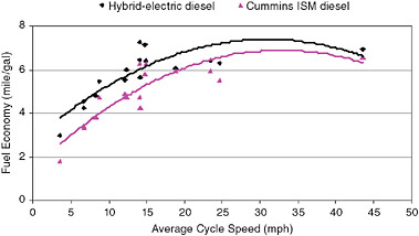
FIGURE 2-15 Curves based on chassis dynamometer for fuel economy versus average speed for conventional and hybrid buses. SOURCE: Wayne et al. (2008). Reprinted with permission from the Transportation Research Forum.
level, a model required to analyze the effects of technologies on fleets (e.g., VOLPE13 and MOBIL614) will be radically different from ones developed to focus on specific vehicles (e.g., PSAT,15 CRUISE,16 RAPTOR,17 ADVISOR,18 and PERE19).
For fleet analysis, average efficiency or fuel consumption gains are usually considered (e.g., VOLPE). In other instances, vehicle fuel consumptions are assumed for specific operating conditions through the use of Bins (e.g., MOBIL6). In all cases, however, the values implemented to assess fleet impacts are generated from more detailed models developed to analyze specific vehicles.
Two main philosophies are used to model specific vehicles: backward-looking model (or vehicle-driven) and forward-looking model (or driver-driven). In a forward-looking model, the driver model will send an accelerator or a brake pedal to the different power train and component controllers (e.g., throttle for engine, displacement for clutch, gear number for transmission, or mechanical braking for wheels) in order to follow the desired vehicle speed trace. The driver model will then modify its command depending on how close the trace is followed. As components react as in reality to the commands, advanced component models can be implemented, transient effects (such as engine starting, clutch engagement/disengagement, or shifting) can be taken into account, or realistic control strategies can be developed that would later be implemented in real-time applications. By contrast, in a backward-looking model, the desired vehicle speed goes from the vehicle model back to the engine to finally find out how each component should be used to follow the speed cycle. Because of this model organization, quasi-steady models can only be used and realistic control cannot be developed. Consequently, transient effects cannot be taken into account. Backward-models are usually used to define trends, while forward-looking models allow selection of power train configurations, technologies as well as development of controls that will later be implemented in the vehicles.
Simulation tools, more specifically forward-looking models that target specific vehicles, are widely used in the industry to properly address the component interactions that affect fuel consumption and performance. With systems becoming increasingly complex, predicting the effect of combining several systems (whether between components or subsystems) is becoming a difficult task due to the nonlinearity of some phenomena.
The models and controls required to accurately model fuel consumption are well defined. For hot conditions and with accurate plant20 data, conventional vehicles can achieve fuel consumptions within 1 to 2 percent compared to dynamometer testing. Advanced vehicles, such as hybrid electric vehicles, are more difficult to validate because the power management system selected by the power train manufacturer has a higher impact on fuel consumption and is subject to many variations as discussed in Chapter 6. The plant models used for fuel consumption are usually based on steady-state look-up tables representing the component losses for different operating conditions. The main datasets are captured from dynamometer testing (e.g., fuel rate for different engine torque/speed points).
Lately, simulation tools have been used to further minimize the time required for the vehicle development process using advanced techniques such as model-based design. Advanced techniques are used to develop/test new control algorithms or plant design, including hardware-in-the-loop (HIL), rapid control prototyping or component-in-the-loop. For example, the component control algorithms are currently developed in simulation using detailed plant models (e.g., GTPower for engine or AMESIM for transmission) and can later be tested using the plant hardware.
To represent any technology properly, such models must be established using the appropriate datasets. One of the critical elements in generating accurate results relies on both selection of the proper level of modeling and collection of the data that will populate the model.
While some phenomena are currently well understood and can be properly modeled (e.g., fuel consumption, performance within 1 or 2 percent), others remain difficult to address properly (e.g., emissions or extreme thermal conditions).
Because criteria emissions cannot be simulated with the fidelity available to simulate fuel consumption and vehicle performance, there can be inherent disconnects and inaccuracies in modeling fuel consumption in an emission-constrained vehicle, meaning all vehicles. For example, engine-off modes that would be used with hybrids might result in lower aftertreatment temperatures and thus lower aftertreatment performance. Without aftertreatment constraints in the simulation, the model might allow engine system operation outside the emission-constrained envelope. At the same time, a hybrid might allow the engine to operate in modes where emissions are lower than they would be in a conventional drive train. More investigation needs to be conducted regarding the influence of fuel consumption reduction technology on actual in-service emissions.
|
13 |
DOT/NHTSA, “Corporate Average Fuel Economy Compliance and Effects Modeling System Documentation,” DOT HS 811 112, April 2009. |
|
14 |
EPA, “The MOVES Approach to Model Emission Model,” CRC On-Road Vehicle Emission Workshop, March 2004. |
|
15 |
|
|
16 |
See www.avl.com. |
|
17 |
SwRI, “RAPTOR Vehicle Modeling and Simulation,” November 2004. |
|
18 |
See www.avl.com. |
|
19 |
EPA, “Fuel Consumption Modeling of Conventional and Advanced Technology Vehicles in the Physical Emission Rate Estimator (PERE),” EPA420-P-05-001, February 2005. |
|
20 |
A “plant” is defined as a system that can be controlled. |
Model-Based Design
Model-based design (MBD) is a mathematical and visual method of addressing the problems of designing complex control systems and is being used successfully in many motion control, industrial equipment, aerospace, and automotive applications. It provides an efficient approach for the four key elements of the development process cycle: modeling a plant (system identification), analyzing and synthesizing a controller for the plant, simulating the plant and controller, and deploying the controller, thus integrating all these multiple phases and providing a common framework for communication throughout the entire design process.
This MBD paradigm is significantly different from the traditional design methodology. Rather than using complex structures and extensive software code, designers can now define advanced functional characteristics using continuous-time and discrete-time building blocks. These built models along with some simulation tools can lead to rapid prototyping, virtual functional verification, software testing, and validation. MBD is a process that enables faster, more cost-effective development of dynamic systems, including control systems, signal processing, and communications systems. In MBD a system model is at the center of the development process, from requirements development, through design, implementation, and testing. The control algorithm model is an executable specification that is continually refined throughout the development process.
MBD allows efficiency to be improved by:
-
Using a common design environment across project teams
-
Linking designs directly to requirements
-
Integrating testing with design to continuously identify and correct errors
-
Refining algorithms through multidomain simulation
-
Automatically generating embedded software code
-
Developing and reusing test suites
-
Automatically generating documentation
-
Reusing designs to deploy systems across multiple processors and hardware targets.
The different phases of MBD are shown in Figure 2-16 (see also Appendix G). The methodology is increasingly being implemented by vehicle manufacturers as part of their vehicle development process. As such, one can envision that some of the same techniques used to accelerate the introduction of new technologies on the market could also be part of the portfolio of options available for regulation. One example is the use of HIL for medium- and heavy-duty-vehicle regulation in Japan. However, one can envision that any step of the MBD approach, from pure simulation to a combination of hardware and software to complete vehicle testing, can be part of the process.
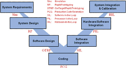
FIGURE 2-16 “V” diagram for software development.
FINDINGS AND RECOMMENDATIONS
Finding 2-1. Fuel consumption (fuel used per distance traveled; e.g., gallons per mile) has been shown to be the fundamental metric to properly judge fuel efficiency improvements from both engineering and regulatory viewpoints, including yearly fuel savings for different technology vehicles. The often-used reciprocal, miles per gallon, called fuel economy, was shown in studies to mislead light-duty vehicle consumers to undervalue small increases (1 to 4 mpg) in fuel economy in lower-fuel-economy vehicles, even though there are large decreases in fuel consumption for small increases in fuel economy. This is because the relationship between fuel economy and fuel consumption is nonlinear. Truck and bus buyers could also likely be misled by using fuel economy data since their fuel economy values are in the lower range (3 to 15 mpg).
Finding 2-2. The relationship between the percent improvement in fuel economy (FE) and the percent reduction in fuel consumption (FC) is nonlinear, and the relationship between change in FE and FC is as follows:
|
% Increase in Fuel Economy |
% Decrease in Fuel Consumption |
|
10 |
9.1 |
|
50 |
33.3 |
|
100 |
50 |
Finding 2-3. Medium- and heavy-duty vehicles are designed as load-carrying vehicles, and consequently their most meaningful metric of fuel efficiency will be in relation to work performed, such as fuel consumption per unit payload carried, which is load-specific fuel consumption (LSFC). Because the main social benefit of trucks and buses is the efficient and reliable movement of goods or passengers, establishing a metric that includes a factor for the work performed will most closely match regulatory with societal goals. Methods to increase payload may be combined with technology to reduce fuel consumption to improve LSFC. Future standards might require different values to accurately reflect the applications of the various vehicle classes (e.g., buses, utility, line haul, pickup, and delivery).
Finding 2-4. Yaw-induced drag can be accurately measured only in a wind tunnel. Standard practice in wind tunnel testing reports a wind average drag (coefficient) that can be 15 percent higher than the drag neglecting yaw.
Finding 2-5.* The large per-vehicle annual miles traveled and fuel use by many heavy-duty vehicles magnify the importance, especially to the user, of technologies or design alternatives that can reduce fuel consumption by as little as 1 percent. As a result, accurate test procedures are required to reliably determine the potential benefit of technologies that reduce fuel consumption. Unfortunately, it is very difficult to achieve, at the 90 or 95 percent confidence interval, a precision of less than ±2 percent for vehicle fuel consumption measurements with the current SAE test procedures. The recently convened SAE Truck and Bus Aerodynamic and Fuel Economy Committee effort is a good start toward developing high-quality industry standards.
Recommendation 2-1. Any regulation of medium- and heavy-duty-vehicle fuel consumption should use load-specific fuel consumption (LSFC) as the metric and be based on using an average (or typical) payload based on national data representative of the classes and duty cycle of the vehicle. Standards might require different values of LSFC due to the various functions of the vehicle classes, e.g., buses, utility, line haul, pickup, and delivery. Regulators need to use a common procedure to develop baseline LSFC data for various applications, to determine if separate standards are required for different vehicles that have a common function. Any data reporting or labeling should state an LSFC value at specified tons of payload.
Recommendation 2-2.* Uniform testing and analysis standards need to be created and validated to achieve a high degree of accuracy in determining the fuel consumption of medium- and heavy-duty vehicles. NHTSA should work with industry to develop robust test and analysis procedures and standards for fuel consumption measurement.
BIBLIOGRAPHY
ANL (Argonne National Laboratory). 2009. Evaluation of Fuel Consumption Potential of Medium and Heavy Duty Vehicles Through Modeling and Simulation
ATA (American Trucking Associations, Inc.). 2007a. Top 100 private carriers 2007. Transport Topics. Available at http://www.ttnews.com/tt100.archive.
ATA. 2007b. Top 100 for-hire fleets 2007. Transport Topics. Available at http://www.ttnews.com/tt100.archive.
ATA. 2009. Top 100 commercial fleets 2009. Light and Medium Truck. July. Available at http://www.lmtruck.com/lmt100/index.asp.
Bradley, M.J., and Associates LLC. 2009. Setting the Stage for Regulation of Heavy-Duty Vehicle Fuel Economy and GHG Emissions: Issues and Opportunities. Washington, D.C.: International Council on Clean Transportation. February.
Chapin, C.E. 1981. Road load measurement and dynamometer simulation using coastdown techniques. SAE Paper 810828. Warrendale, Pa.: SAE International.
Clark, N.N., M. Gautam, W.S. Wayne, R.D. Nine, G.J. Thompson, D.W. Lyons, H. Maldonado, M. Carlock, and A. Agrawal. 2003. Creation and evaluation of a medium heavy-duty truck test cycle. SAE Transactions: Journal of Fuels & Lubricants, Vol. 112, Part 4, pp. 2654-2667.
Clark, N.N., M. Gautam, W. Riddle, R.D. Nine, and W.S. Wayne. 2004. Examination of a heavy-duty diesel truck chassis dynamometer schedule. SAE Paper 2004-01-2904. SAE Powertrain Conference, Tampa, Fla., Oct.
Clark, N.N., M. Gautam, W.S. Wayne, D.W. Lyons, and G.J. Thompson. 2007. Heavy-duty vehicle chassis dynamometer testing for emissions inventory, air quality modeling, source apportionment and air toxics emissions inventory. Coordinating Research Council, Inc. Report No. E-55/59, Available at http://www.crcao.com/reports/recentstudies2007/E-55-59/E-55_59_Final_Report_23AUG2007.pdf. Accessed July 8, 2009.
CRC (Coordinating Research Council), March 2002. Qualification of the Heavy Heavy-Duty Diesel Truck Schedule and Development of Test Procedures. Final Report, CRC Project E-55-2.
Davies, C., J. Findsen, and L. Pedraza 2005. Assessment of the Greenhouse Gas Emission Benefits of Heavy Duty Natural Gas Vehicles in the United States. Final Report, September 22. Prepared for the U.S. Department of Transportation, Center for Climate Change and Environmental Forecasting, Washington, D.C.
Davis, S., and S. Diegel. 2007. Transportation Energy Data Book Edition 26. Oak Ridge, Tenn.: Oak Ridge National Laboratory.
DOE/EERE (U.S. Department of Energy/Office of Energy Efficiency and Renewable Energy). 2009. 2008 Vehicle Technologies Market Report. Golden, Colo.: National Renewable Energy Laboratory. July. Available at http://www.nrel.gov/docs/fy09osti/46018.pdf.
EPA (U.S. Environmental Protection Agency). 2004. The MOVES Approach to Model Emission Model. Presentation to the Coordinating Research Council’s 14th On-Road Vehicle Emission Workshop, San Diego, Calif., March 29-31. Available at http://www.epa.gov/otaq/models/ngm/may04/crc0304a.pdf.
EPA (U.S. Environmental Protection Agency). 2009. SmartWay Truck Emissions Test Protocol Workshop. Drive Cycle Development. Available at http://www.epa.gov/SmartWayshipper/transport/documents/tech/drive-cycle-development.pdf. Accessed September 22, 2009.
Frey, C., and J. Zheng. 2002. Probabilistic analysis of driving cycle-based highway vehicle emission factors. Environmental Science and Technology, Vol. 35 (23), October 30, pp. 5184-5191.
Gautam, M., N.N. Clark, W. Riddle, R. Nine, W.S. Wayne, H. Maldonado, A. Agrawal, and M. Carlock. 2002. Development and initial use of a heavy duty diesel truck test schedule for emissions characterization. SAE Transactions: Journal of Fuels & Lubricants, Vol. 111, pp. 812-825.
Gaylard, A.P. 2009. The appropriate use of CF in the automotive design process. SAE Paper 2009-01-1162. Presented at the SAE World Congress and Exhibition, Detroit, Mich. April.
Gaylard, Adrian Philip. The appropriate use of CFD in the Automotive Design Process, SAE 2009-01-1162. April 2009.
Graboski, M.S., R.L. McCormick, J. Yanowitz, and L. Ryan. 1998. Heavy-duty diesel vehicle testing for the northern front range air quality study. Fort Collins, Colo.: February.
Larrick, R.P., and J.B. Soll. 2008. The MPG illusion. Science, Vol. 320, June 20.
Metro Magazine. 2009. 2009 Fact Book.
Nam, E. 2009. Drive cycle development and real-world data in the United States: Why drive cycles are important. Presentation by the U.S. Environmental Protection Agency at WLTP meeting Geneva, January 15.
Nine, R.D., N.N. Clark, and P. Norton. 2000. Effect of emissions on multiple driving test schedules performed on two heavy duty vehicles. SAE Paper 2000-01-2818. Fall Fuels and Lubricants Meeting and Exposition, Baltimore, Md. October.
SAE (Society of Automotive Engineers) Standards, Procedures, and Recommended Practices. Warrendale, Pa.: SAE International.Various years:
SAE J1082. Fuel Economy Measurement Road Test Procedure. February 2008.
SAE 1252. SAE Wind Tunnel Text Procedure for Trucks and Buses. Warrendale, Penn.: SAE International. July 1981; update in progress.
SAE J1263. Road Load Measurement and Dynamometer Simulation Using Coastdown Techniques. January 2009.
SAE J1264. Joint Rccc/SAE Fuel Consumption Test Procedure (Short Term In-Service Vehicle), Type I. October 1986; update in progress.
SAE J1321. Joint Tmc/SAE Fuel Consumption Test Procedure—Type II. October 1986; update in progress
SAE J1376. Fuel Economy Measurement Test (Engineering Type) for Trucks and Busses. July 1982.
SAE J1711. Recommended Practice for Measuring the Exhaust Emissions and Fuel Economy of Hybrid-Electric Vehicles. March 1999; update in progress.
SAE J2263. Road Load Measurement Using Onboard Anemometry and Coastdown Techniques. December 2008.
SAE J2264. Chassis Dynamometer Simulation of Road Load Using Coast-down Techniques. April 1995; update in progress.
SAE J2452. Stepwise Coastdown Methodology for Measuring Tire Rolling Resistance. June 1999; update in progress.
SAE J2711 Recommended Practice for Measuring Fuel Economy and Emissions of Hybrid-Electric and Conventional Heavy-Duty Vehicles. September 2002.
Thompson, G.J., N.N. Clark, R.J. Atkinson, Z. Luzader, F.L. Vanscoy, V. Baker, and J. Chandler. 2004 Development of an interface method for implementing road grade in chassis dynamometer testing. American Society of Mechanical Engineers (ASME) Paper ICEF2004-896. Internal Combustion Engine Division 2004, ASME Fall Technical Conference, October 24-27, Long Beach, Calif.
TMA (Truck Manufacturers Association). 2007. Test, Evaluation, and Demonstration of Practical Devices/Systems to Reduce Aerodynamic Drag of Tractor/Semitrailer Combination Unit Trucks. Contract Number DE-FC26-04NT42117. National Energy Technology Laboratory, Morgantown, W.Va. April.
Walkowicz, K. 2006. Testing and evaluation of the GM/Allison Hybrid System in the King County Metro Transit Fleet. Presentation to the APTA Bus and Paratransit Conference, Seattle, Wash., May.
Wang, W., M. Gautam, X. Sun, R. Bata, N.N. Clark, G.M. Palmer, and D.W. Lyons. 1994. Emission comparisons of twenty-six heavy duty vehicles operated on conventional and alternative fuels. SAE Transactions, J. Commercial Vehicles, Vol. 102, Section 2, pp. 31-40.
Wang, W., D.W. Lyons, R. Bata, N.N. Clark, and M. Gautam. 1995. Inuse emissions tests of alternatively fueled heavy-duty vehicles with a transportable chassis dynamometer. Proc. Inst. Mech. Eng., Part D., J. Automobile Engineering, Vol. 209.
Wayne, W.S., N.N. Clark, A.B.M.S. Khan, M. Gautam, G.J. Thompson, and D.W. Lyons. 2008. Regulated and non-regulated emissions and fuel economy from conventional diesel, hybrid-electric diesel and natural gas transit buses. Journal of the Transportation Research Forum, Vol. 47, No. 3, October, pp. 105-126.


