
4
Physical Climate Change in the 21st Century
4.1
REGIONAL PATTERNS OF WARMING AND RELATED FACTORS
An approximation on which we will rely in this report is “pattern scaling”, in which a robust pattern of climate change is assumed to exist that describes the geographical and seasonal structure of the temperature response that does not depend on climate sensitivity or on details of the forcing or emission scenario. All of the scenario and sensitivity dependence is captured within the time evolving global mean surface temperature, TG(t). Letting the symbol ξ stand for the two horizontal spatial coordinates and the time of year, the assumption is that
The pattern τ(ξ) has a spatial-annual mean of unity by definition. We focus on temperature here and discuss pattern scaling for precipitation in Section 4.2.
The validity of this approximation is discussed by Santer et al. (1990), Mitchell et al. (1999), and Mitchell (2003). It has been used extensively for regional temperature (and precipitation) change projections (Dessai et al., 2005; Murphy et al., 2007; Watterson, 2008) and impacts studies, as a substitute to running fully coupled simulations under different scenarios or with different models with a range of climate sensitivities.
The pattern is derived from experiments with fully coupled Global Climate Models (GCMs), with validation from efforts to isolate the well-mixed greenhouse gas signal from the historical temperature record. The value of the method relies on the pattern remaining fairly constant during a simulation, across different concentration pathway scenarios and across different model settings. Regionally and temporally differentiated results under different scenarios or climate sensitivities can be derived by first characterizing the stable geographical pattern of warming (and its spatial variability
if some measure of uncertainty is sought) on the basis of available coupled model simulations, then adjusting the profile of transient warming by using a fast and simple energy balance model to predict the global mean surface temperature evolution. There are significant differences between the patterns generated by different models—for example, in the amount of polar amplification in the Arctic per degree of global warming. These differences are averaged over in the ensemble-based estimates of mean patterns, but uncertainty can be characterized by the inter-model spread in the pattern τ(ξ).
The choice of the pattern in the studies available in the literature are often as simple as the ensemble average (across models and/or across scenarios, for the coupled experiments available) of the spatial change in temperature, normalized by the corresponding change in global average temperature, choosing the end of the simulations (usually last two decades of the 21st century) and a baseline of reference (pre-industrial or current climate). Similar properties and results have been obtained using more sophisticated multivariate procedures that optimize the variance explained by the pattern.
There are limitations to this approach. It can break down if aerosol forcing is significant, not only because aerosols and greenhouse gases can have different spatial footprints, but also because the effects of aerosols themselves are more difficult to characterize in this simple way. For example, Asian and North American aerosol production are likely to have different time histories in the future. Our focus in this report is on the greenhouse gas component of climate change, making the pattern scaling assumption more justifiable.
Simple pattern scaling is regarded as especially useful for summarizing model projections of transient climate change due to well-mixed greenhouse gas increases on a time scale of a few centuries. But it is less accurate for stabilization scenarios, as the temperature changes approach an equilibrium response. From the early work of Manabe and Wetherald (1980) and Mitchell et al., (1999) it has been clear that the pattern of temperature response evolves as the slow component of the warming, associated with equilibration of the deep oceans on multi-century time scales, equilibrates. In particular, on these long time scales the warming of high latitudes in the Southern Hemisphere is much larger relative to the global mean warming than in the earlier periods. Held et al. (2010) emphasize that this slow warming pattern is present, but of small amplitude, during the initial transient adjustment phases of the response as well.
There are some regions of sharp temperature gradients, near the ice edge
for example, where pattern scaling will break down. As the climate warms, temperature changes will be large as the ice edge moves across a particular location, but then return to small values with additional warming, because the ice edge is now further poleward.
Given other uncertainties, we find that pattern scaling is justified for current attempts to link stabilization targets and impacts, keeping in mind limitations due to the evolution of the pattern of warming on long, stabilization time scales and the limitations in regions of sharp gradients.
On the basis of CMIP3 simulations, Chapters 10 and 11 of IPCC AR4, WG1 analyzed geographical patterns of warming and measures of their variability across models and across scenarios. The executive summary of Chapter 10 reports that “[g]eographical patterns of projected SAT warming show greatest temperature increases over land (roughly twice the global average temperature increase) and at high northern latitudes, and less warming over the southern oceans and North Atlantic, consistent with observations during the latter part of the 20th century …”. Figure 10.8 of the report depicts the patterns of annual average warming across three scenarios (A2, A1B and B1) and three time periods (2011-2030, 2046-2065, and 2080-2099) over which change is computed. Figure 10.9 shows seasonal patterns for DJF and JJA under A1B. Chapter 10 also reports that the spatial correlation of fields of temperature change is as high as 0.994 in the model ensemble mean when considering late 21st century changes between A2 and A1B. A table in the same section (Table 10.5) quantifies the strict agreement between the A1B field, as a standard, and the other scenario patterns using a measure proposed by Watterson (1996) with unity meaning identical fields and zero meaning no similarity. Values of this measure are consistently above 0.8 and increase as the projection time increases (later in the 21st century fields agree better than earlier in the century), with values of 0.9 or larger for the late 21st century. The same table also shows that the agreement deteriorates if considering commitment scenarios. The results are documented as applying to seasonal warming patterns besides annual averages.
On the basis of the previous discussion and results, we compute patterns of standardized warming from the available CMIP3 SRES scenario simulation and produce maps of the ensemble average warming (these—in their non-normalized version—are available from AR4 WG1 Figures 10.8 and 10.9, and individual models’ maps are available in supplementary material in Chapter 10 (http://ipcc-wg1.ucar.edu/wg1/Report/suppl/Ch10/Ch10_indiv-maps.html, and Chapter 11 (http://www.ipcc.ch/pdf/assessment-report/ar4/wg1/ar4-wg1-chapter11-supp-material.pdf) along with measures of the regionally differentiated variability of this pattern across models and scenarios (IPCC, 2007a).
Figure 4.1 shows patterns of warming normalized “per degree C of global annual average warming”. Ranges across models or across scenarios are shown in Figures 4.4 and 4.5. We show maps of global geographical patterns and North American patterns for annual average warming and December-January-February and June-July-August average warming.
We highlight here the main features characterizing warming patterns:
The annual and DJF mean patterns present a typical gradient of warming that decreases from north to south, with the higher latitude of the Northern Hemisphere seeing the largest increases, and the land masses warming more than the oceans. The JJA patterns’ main characteristics are an enhanced warming of the interior of the continents and the Mediterranean Basin, with a gradient that is generally equator to poles rather than north-south. The largest source of variation resides in the inter-model spread rather than the inter-scenario spread, and it is mainly localized over and at the edge of the ice sheets of the Arctic and Antarctica.
We also present in Figure 4.2 a number of scatter plots depicting the relation between the magnitude of global average warming (by 2080-2099 compared to 1980-1999) and the magnitude of regional warming across models (each model one dot) and scenarios (color-coded) for several of the “Giorgi regions” (Giorgi and Francisco, 2000). We chose four regions that subdivide the North American continent (western, central, and eastern North America—WNA, CNA, and ENA respectively—and Alaska, ALA) plus two regions in other climates for comparison, the Mediterranean Basin (MED) and Southern Australia (SAU). The linearity of the relationship and the fairly tight spread around it is clear. As already noted, the source of variation between different models is larger than from the scenarios: averaging each model across the three scenarios would not reduce the scatter as much as averaging all the models within one scenario, as shown by the larger star-shaped marks.
Finally, in Figure 4.3 we show December-January-February and June-July-August warming patterns as calculated in models including both anthropogenic and natural forcing for the 20th century, together with 20th century observations. Figure 4.3 shows that the warming patterns in the models and observations display many common large-scale features, and a comparison with Figure 4.1 demonstrates how 20th century patterns contain already many of the large-scale features that characterize 21st century patterns. Among these, the relatively larger magnitude of the warming in December-January-February than in June-July-August in both observed and modeled patterns; the amplification of the warming in the high latitudes of the Northern Hemisphere characteristic of December-January-February
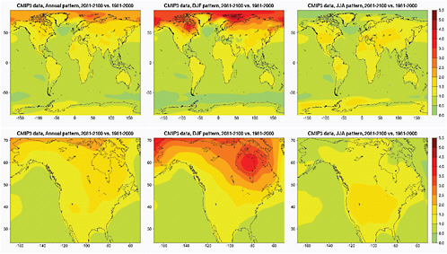
FIGURE 4.1 Geographical patterns of warming per 1°C of global annual average warming, over the whole world (top) and over North America (bottom). From left to right: patterns for average temperature over the whole calendar year or for average temperature in boreal winter (December, January, and February) or summer (June, July, and August). Patterns are obtained by scaling end-of-21st-century changes (compared to end-of-20th-century climatology) by global average annual warming over the same period, using temperature at the surface from the 18 CMIP3 models whose output is available for SRES scenarios A2, A1B, and B1.
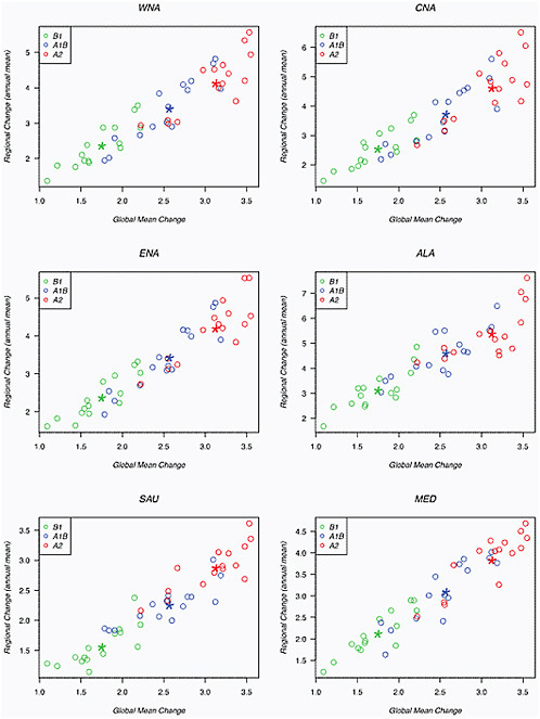
FIGURE 4.2 Scatterplots comparing regional average warming versus global average warming (both averaged over the calendar year) for western North America (WNA), central North America (CNA), eastern North America (ENA), Alaska (ALA), Southern Australia (SAU) and the Mediterranean (MED). Each point indicates results from an individual model under one of the three SRES scenarios (A1B, blue; A2, red; and B1, green). Stars indicate the multi-model ensemble averages for each of the three scenarios.
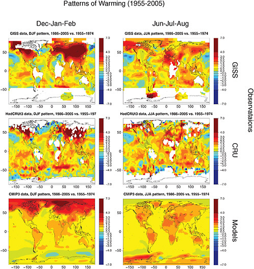
FIGURE 4.3 Relative patterns of warming (normalized to one for the globe),for December-January-February (left) and June-July-August (right) for 1955-2005 (obtained as differences between 20-year average temperatures for 1986-2005 and 1955-1974). The top two panels show results from two instrumental temperature records, NASA GISS and CRU. White indicates regions where data are not available. The bottom panels show results for the Climate Modelling Intercomparison Project (CMIP3) multi-model ensemble. Patterns expected from projections for the 21st century are largely similar to those shown here, as seen in Figure 4.1.
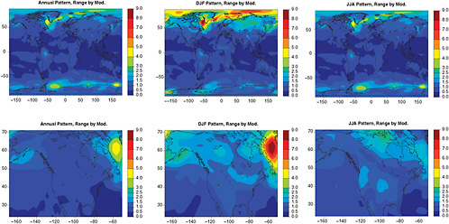
FIGURE 4.4 For the same patterns as in Figure 4.1, the range across the 18 models of the average of each model’s patterns obtained under the three different scenarios is shown as a measure of the variability of the patterns produced by different GCMs.
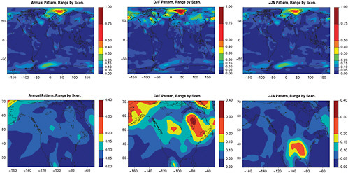
FIGURE 4.5 For the same patterns as in Figure 4.1, the range across SRES A1B, A2, and B1 of the patterns derived as a multi-model ensemble is shown as a measure of the variability of the patterns under different emission scenarios.
warming; and the strong signal of warming in the semi-arid to arid regions especially in the Mediterranean basin and nearby portions of the Asian continent in June-July-August. Areas of disagreement between models and observations remain, particularly in the form of more homogeneous patterns of warming at the subcontinental scales in the modeled patterns than in observations, with one example being the area of cooling in the southeast of the United States appearing in the HadCRU data and not represented in the models.
4.2
PRECIPITATION RESPONSE
As described in Section 4.1, it is reasonable to assume that the local temperature response to an increase in a well-mixed greenhouse gas is proportional to the global mean temperature response, with a well-defined spatial and seasonal pattern. There are also good reasons to assume that the local precipitation response scales with the global mean surface temperature response, although the uncertainties are greater, both with regard to the spatial and seasonal structure of the pattern and with regard to the limitations of this pattern scaling assumption.
Using the CMIP3 archive and computing the precipitation response, measured as a percentage change, divided by the global mean warming and then averaging over models and scenarios, just as for the temperatures in Figure 4.1, one obtains the pattern shown in Figure 4.6, both globally for the annual average and the summer and winter seasons, and focusing on North America (which is not found in the IPCC AR4 report [IPCC, 2007a]). The patterns are very similar to those shown for a particular scenario and time frame in the Summary for Policy Makers of the AR4/WG1 report (IPCC, 2007e).
There is a general increase in precipitation in subpolar and polar latitudes, and a decrease in the subtropics, and an increase once again in many equatorial regions. The boundary between the subtropical decrease and subpolar increase cuts through the continental United States, but with the boundary moving north in the summer and south in the winter. As a result, this ensemble mean projection is for an increase in precipitation in much of the continental United States in the winter and a reduction in the summer. In contrast, Canada is more robustly wetter and Mexico drier, being located closer to the centers of the subpolar region of increasing precipitation and the subtropical region of decreasing precipitation, respectively. The Mediterranean/Middle East and southern Australia are other robust regions of drying in these projections.
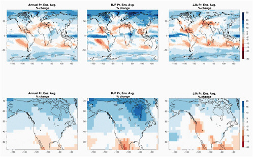
FIGURE 4.6 Geographical patterns of percentage precipitation change per 1°C of global annual average warming, for the whole world (top) and over North America (bottom). From left to right: patterns of changes in precipitation averaged over the whole calendar year or over boreal winter (December, January, and February) or summer (June, July, and August). Patterns are obtained by scaling end-of-21st-century percentage changes in precipitation (compared to end-of-20th-century climatology) by global average annual *warming* over the same period for the 18 CMIP3 models whose output is available for all three SRES scenarios A2, A1B, and B1. White regions are where less than two-thirds of the models agree over the sign of the change.
Focusing on fixed seasons provides one snapshot into these projected patterns. An alternative procedure, emphasizing the extent to which the “dry get drier”, is to plot the precipitation changes in the driest 3 months at each location, irrespective of calendar date (Solomon et al., 2009). This alternative version is provided in the section, “Overview of Climate Changes and Illustrative Impacts.” Local details differ, but the large-scale pattern is unchanged.
Our confidence in this model-generated pattern is enhanced by an understanding of the simple underlying mechanism controlling its structure. The starting point on which this understanding is based is the increase in the saturation pressure for water vapor with increasing temperature. Most of the water vapor in the atmosphere resides in the lowest 2-3 Km, where the saturation vapor pressure increases at roughly 7% per 1ºC of warming. The ratio of water vapor in the atmosphere to this saturation value is referred to as the relative humidity. Especially near the surface, observational trends (e.g, Trenberth et al., 2005) and simple physical arguments (Held and Soden, 2006) consistently show that relative humidity cannot be expected to change substantially on average, and certainly not enough to counterbalance the increase in water vapor expected from the increase in saturation vapor pressure. As a result, there is high confidence in the projection that the total water vapor in the atmosphere will increase at roughly 7% per 1ºC of warming.
If one averages around latitude circles, the hydrological cycle on Earth can be pictured schematically as in Figure 4.7. Evapotranspiration is largest in lower latitudes and decreases steadily as one moves poleward. Precipitation is larger than evapotranspiration in subpolar latitudes, and near the equator, and less than evapotranspiration in the subtropics. Fluxes of water vapor in the atmosphere are responsible for these local excesses and deficits. The atmosphere is converging water into the regions of excess and diverging water from the regions of deficit. As temperature increases and the amount of water vapor increases, the divergence and convergence of the water vapor flux increase proportionally, increasing the magnitudes of these excesses and deficits This simple picture also explains the magnitude of the increases and decreases in precipitation expected: because water vapor increases by roughly 7% per 1ºC, the atmospheric fluxes increase by the same percentage, so that the pattern of precipitation minus evaporation is also amplified by about the same factor.
The final element in the picture is that the changes in the global mean hydrological cycle, the globally averaged precipitation and evapotranspiration, increase more slowly than do the increase in these water vapor fluxes.
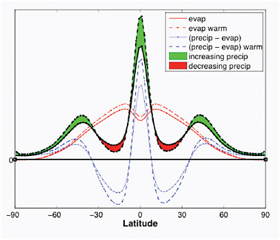
FIGURE 4.7 A schematic of the precipitation P (black) and evapotranspiration E (red) and P-E (blue) averaged around latitude circles. Solid lines indicate the unperturbed climate, and dotted lines a warmer climate. E increases slightly but is overwhelmed, on average, by the increase in magnitude of P-E, which is controlled by the magnitude of the horizontal water vapor fluxes.
The increase in precipitation in subpolar latitudes, for example, is due to an increase in the flux of vapor into these latitudes and not primarily to an increase in evaporation.
This picture is conservative, in that it assumes that changes in the atmospheric circulation are small so that the fluxes of vapor are dominated by the increases in the vapor itself and not in the winds carrying the vapor. This assumption has to be modified to understand model projections in more detail (see Section 4.4).
In the tropics the circulation is primarily driven by the heat released where water vapor condenses, so one cannot assume that the tropical winds will remain the same as water vapor increases. Partly due to the complexity of the interactions between winds and rainfall in the tropics, model projections for changes in rainfall are not as robust as in other areas. Some models predict dramatic drying of the Amazon, with important consequences for the forest and the global carbon cycle, but other models do not. Some models
predict dramatic dying in parts of sub-Saharan Africa, but others do not. Patterns of precipitation changes in middle and higher latitudes are more robust on large scales but remain uncertain on the regional scales of importance for impact and adaptation strategies. For example, the changes in precipitation in the western United States in wintertime are sensitive to the El Niño phenomenon in the equatorial Pacific, the response of which is itself uncertain. And especially over semi-arid land surfaces, arguments based on the assumption that relative humidities do not change can break down. Given these complexities, we consider the CMIP3 ensemble as providing our best estimates of the pattern of precipitation change accompanying global warming, with consistency or inconsistency across this ensemble provided some indication of uncertainties.
4.3
HURRICANES
Atlantic Hurricanes
Atlantic hurricane activity has increased markedly in the past 20 years, concurrent with increases in ocean temperatures in the tropical North Atlantic region in which hurricanes are formed. But it is well established that hurricane frequency is dependent on other aspects of the large-scale climate as well as the local ocean temperatures. Many of the issues regarding detection, attribution, and projection of tropical cyclone trends in the Atlantic and throughout the tropics have recently been assessed by a WMO expert team (Knutson et al., 2010). We highlight a few of these issues here, basing the discussion in large part on this recent assessment, and refer the reader to Knutson et al. (2010) for a more detailed discussion.
Several detailed studies of the tropical storm record in the Atlantic have converged on a consensus view that the recent trend is more likely due to internal multi-decadal variability than a part of a century-long trend associated with greenhouse gas increases. While the raw data for Atlantic storms suggest a significant century-long trend, three separate lines of analysis cast doubts on the reality of this trend: (1) the frequency of landfalling storms, for which the completeness of the data is less of an issue than for basin-wide statistics, shows no significant long-term trend (Landsea, 2007); (2) estimates based on historical ship tracks indicate enough storms were likely missed in the early part of the century to account for most of the long-term trend in storm frequency (Chang et al., 2007; Vecchi and Knutson, 2008); and (3) the long-term trend in the raw data is primarily from short-lived storms (<3 days), which also suggests data artifacts are dominating the long-term
trend (Landsea et al., 2010). The tentative picture that emerges is of Atlantic cyclone frequency being strongly modulated by internal multi-decadal variability, with levels of activity as high in the mid-20th century and the late 19th century as in the most recent decade. Additional clarification of tropical cyclone records outside of the Atlantic are needed to provide a clearer global picture of trends and variability.
Recent studies with relatively high-resolution global atmospheric models and with dynamical and statistical downscaling techniques have supported this picture. Several of these studies have successfully simulated the trend in Atlantic storm frequency in recent decades when provided with boundary conditions, especially ocean temperatures, as observed over this period (Knutson et al., 2008; LaRow et al., 2008; Zhao et al., 2009). When these or similar models are used to simulate the tropical storm statistics consistent with climate projections for the late 21st century, they consistently predict responses that cannot be obtained by extrapolating recent Atlantic frequency trends (e.g., Sugi et al., 2002; Oouchi et al., 2006; Bengtsson et al., 2007; Knutson et al., 2008; Zhao et al., 2009). Averaged over the globe, models typically predict that the frequency of tropical cyclones will stay roughly unchanged or be reduced by 0-10% per degree C global warming. Within the Atlantic basin, there is more variance in the results, with projections either increasing or decreasing frequencies by as much as 25% per degree C global warming.
New high-resolution studies are appearing regularly, so this picture is likely to evolve, but results to date suggest that the recent increase in Atlantic activity is likely due to an increase in tropical Atlantic ocean temperatures relative to the rest of the tropics and not to the absolute increase in temperatures (i.e., Vecchi et al., 2008). Consistently, the spread in projections for the future may have less to do with the details of the downscaling approach and more to do with the spatial pattern of tropical ocean warming projected by different global climate models, with those models that project larger (smaller) warming in the Atlantic than in other ocean basins resulting in an increase (decrease) in Atlantic storm activity (Zhao et al., 2009).
Insights into likely changes in storm intensity are primarily guided by the theory of the maximum intensity that tropical cyclones can attain in a given environment (Emanuel, 1987), by idealized modeling studies (Knutson and Tuleya, 2004), and a small number of attempts at dynamical and statistical downscaling (Emanuel et al., 2008). A consensus picture emerges in which storms are expected to become more intense on average, roughly by 1-4% per degree global warming, as measured by maximum wind speeds (Knutson et al., 2010), or by 3-12% per degree for the cube of this wind speed, of-
ten taken as a rough measure of the destructive potential of storm winds (Knutson et al., 2010). Whether the frequency of the most intense (category 3-5) cyclones should be expected to increase is less certain, in that it is also affected by the potential for reduction in total cyclone numbers.
An increase in rainfall within tropical cyclones is projected by arguments based on the increase in atmospheric water vapor. Typical values in models are on the order of an 8% increase per degree warming for the rainfall within 100 km of the storm center (Knutson et al., 2010).
4.4
CIRCULATION AND RELATED FACTORS
As discussed in Section 4.2, increasing greenhouse gas concentration is expected to cause an increase in atmospheric moisture of about 7% per degree C global temperature increase. In general, this will lead to greater rainfall in the tropical monsoon regions and drier conditions in the subtropical regions. Wet regions over the tropical oceans should also see increases in precipitation, although the positioning of these centers may shift due to coupled atmosphere-ocean interactions. The increase in atmospheric moisture is also expected to increase precipitation in the mid-latitude storm track regions by roughly 5-10% per degree C global temperature increase; however, it is not clear that storminess will increase.
Arguments based on first principles also indicate that increasing greenhouse gas concentrations should cause the mid-latitude jets and attendant storm tracks to shift poleward (e.g., Hartmann et al., 2000). Since in the atmosphere the temperature increase due to increasing greenhouse gases is confined to the troposphere and the tropopause is higher in the tropics than in high latitudes, increased greenhouse gases causes the poleward pressure gradient at the tropopause in mid-latitudes to increase. This, in turn, causes changes in the wave-mean flow interactions that shift the jets and their associated storm tracks poleward. This poleward shift in the jets and stormtracks should persist as long as the greenhouse gas concentrations remain elevated. A poleward shift in the jets and stormtracks due to global warming is a robust feature of the climate models (Miller et al., 2006; Hegerl et al., 2007; Meehl et al., 2007), with a zonal mean poleward shift of about 100 km per 3ºC global temperature increase.
As a result of the poleward shift in the storm tracks, precipitation will likely increase on the poleward—and decrease on the equatorward side—of the location the climatological jets in the present climate. As noted in Section 4.2, this is indeed the pattern of precipitation change that is found across
western North America in summertime when greenhouse gas concentrations are enhanced.
The same argument for a poleward shift in the storm tracks in the Northern Hemisphere in a warmer climate also applies in the Southern Hemisphere. Because the jet and storm tracks are intimately related and in the southern hemisphere they are circumpolar and vary weakly with longitude, this pattern of climate change is called the Southern Annular Mode (SAM; named after the leading pattern of circulation variability in the Southern Hemisphere due to wave-mean flow interactions—largely in the troposphere). There is ample evidence that the SAM-like changes in the mid- and high-latitude circulation in the Southern Hemisphere that were observed in the latter third of the 20th century (a poleward shift in the jet) was in part due to the human-induced depletion of stratospheric ozone (see, e.g., Miller et al., 2006 and references therein). Hence, a poleward shift in the jet in the Southern Hemisphere that would otherwise be expected because of increasing greenhouse gases will be somewhat tempered until about mid-21st century—when the stratospheric ozone is expected to be nearly recovered.
Many of the AR4 climate models forced by increasing greenhouse gases show that the Meridional Overturning Circulation (MOC) in the Atlantic Ocean will slow down over the 21st century in direct response to increased buoyancy in the sinking regions of the North Atlantic (Meehl et al., 2007). The increased buoyancy is due to both warming and freshening, with the former being more important than the latter. The slowdown in the MOC will have several impacts including a somewhat muted change in surface temperature in the North Atlantic and in maritime western Europe compared to other oceanic regions and modifications in the gradients in tropical sea surface temperature, which will further influence hurricane activity in the tropical Atlantic. The poleward movement of the jet in the Southern Hemisphere will cause the Antarctic Circumpolar Current to narrow and shift southward, impacting the sea-ice extent, the temperature of the water in contact with the floating ice sheets, and the exchange of carbon between the atmosphere and ocean.
There is much interest in knowing, as the planet warms: “How will the El Niño/Southern Oscillation (ENSO) and its teleconnected climate impacts change?” Unfortunately, this question cannot as yet be answered with confidence because almost all of the present climate models have poor representations of ENSO—as measured by the incongruities between the observed and simulated spatial and temporal characteristics of the observed ENSO and those simulated by the climate model. These nature-model incon-
sistencies likely result from the rather large biases in the climatology of the atmosphere and ocean in the tropical Pacific in current generation of global climate models (e.g., the double Intertropical Convergence Zone (ITCZ) common to many of the models). Whether or not the spatial, temporal and amplitude characteristics of ENSO change in a warmer world, however, the associated far-field impacts of ENSO will be different for several reasons. For example, the pattern and amplitude of the mid-latitude wintertime climate anomalies associated with ENSO will change as the mid-latitude jets shift poleward; places that experience drought during the warm (Australia) or cold (central United States) phase of ENSO and that are projected to dry with increasing global average temperature will experience enhanced drought conditions associated with identical ENSO cycles.
4.5
TEMPERATURE EXTREMES
The literature on temperature (as well as that on precipitation) extremes clearly suggests that any method trying to link changes in extremes of maximum and/or minimum temperature, and their consequent effects on the number of very hot or very cold days, and on the duration of hot and cold spells, to global or even local average temperature changes would fall short. As a recent indication of this, a paper by Ballester et al. (2010) shows how an accurate scaling of temperature extremes would have to involve not only average temperature change under future scenarios, but also change in temperature variability and in the skewness of its distribution. No paper has addressed explicitly the quantitative differences across multiple scenarios (or stabilization targets) of temperature extremes that we could straightforwardly utilize to describe expected changes under different atmospheric concentrations.
We chose here to adopt the perspective offered by Battisti and Naylor (2009)—BN09 from now on—on the expected changes in the likelihood of experiencing extremely hot or unprecedented average summer temperatures. This way of characterizing warming from the perspective of the tail of the distribution of average temperature has the strength of utilizing model output (seasonal averages of surface temperature, or TAS) whose reliability has been more extensively corroborated than other parameters representing more traditional definitions of extreme or rare events (e.g., daily temperatures exceeding high thresholds). We adapt BN09’s analysis to our report’s focus on different stabilization targets and make it consistent with its reliance on pattern scaling in order to infer geographically detailed projections of temperature changes as a linear function of changes in global average temperature (see Methods, Section 4.5).
Maps similar to those in Figure 3 of BN09 will result from each shift in mean temperature, except they will correspond to different atmospheric concentrations of CO2 (and their implied expected global average warming) rather than to different future periods. The main difference in our approach compared to the analysis in BN09 is the choice of shifting the distribution uniformly to the right rather than trying to build a new distribution of average temperature anomalies on the basis of model output. This is a choice dictated by the use of pattern scaling, which lacks the availability of an ensemble of fully coupled model runs for each CO2 target.
It could be argued that our analysis represents a conservative estimate of the expected changes in extreme seasonal temperatures, because we are assuming no change in the climatological distributions of temperatures besides a shift of their central locations. In particular, no change in the variability of seasonal average temperature is taken into consideration. Some studies (see for example Scherrer et al., 2005; Fischer and Schar, 2009 for the European region; Giorgi and Bi, 2005; Kitoh and Mukano, 2009 for global patterns) have shown that future variability of summer temperature is projected to increase, in association with drying.
In Figures 4.8 and 4.9 we show the resulting likelihoods of exceeding the 95th percentile, or the warmest anomaly of current average JJA and DJF temperatures (1971-2000 of 20C3M simulations) for the three levels of global warming. The patterns become redder (higher likelihood) as we look down each column (larger global average warming implies greater chances of exceeding the thresholds) and bluer (smaller likelihood) as we look across rows (higher thresholds make exceedances rarer).
4.6
PRECIPITATION EXTREMES
A general increase in atmospheric water vapor is predicted by essentially all climate models as temperatures increase, and an upward trend in column integrated water vapor has been observed in many regions (Trenberth et al., 2005). The consequences of this increase for the distribution of mean precipitation has been discussed in Section 4.2. As outlined below, models and simple theories also suggest that this increase in water vapor will increase the intensity of heavy rainfall events. Increasing trends in extreme precipitation have been documented in many regions, including much of North America (USCCSP, 2008c), but evidence for associated increases in floods is not compelling to date (Lins and Slack, 1999, 2005; WWAP, 2008).
As articulated by Trenberth (1999) and many others, precipitation in storms is related mostly to atmospheric moisture convergence rather than
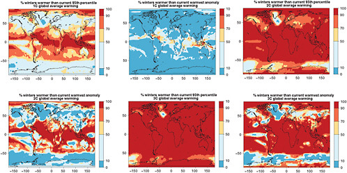
FIGURE 4.8 Chances that December-January-February average temperatures will be warmer than the 5th percentile of the climatological distribution (1971-2000)—left column—and warmer than the warmest (boreal) winter in the climatological distribution—right column—for different degrees of global annual average warming (1°C, 2°C, and 3°C ,respectively, along the three rows). Global average warming is calculated with respect to 1971-2000 averages. To obtain warming with respect to pre-industrial add 0.8°C.
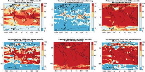
FIGURE 4.9 Chances that June-July-August average temperatures will be warmer than the 5th percentile of the climatological distribution (1971-2000)—left column—and warmer than the warmest (boreal) summer in the climatological distribution—right column—for different degrees of global annual average warming (1°C, 2°C, and 3°C, respectively, along the three rows). Global average warming is calculated with respect to 1971-2000 averages. To obtain warming with respect to pre-industrial add 0.8°C.
evapotranspiration during the storm; therefore, a storm with a given structure (with given vertical motion in particular), will generate more precipitation in a warmer climate, roughly following the increase in saturation vapor pressure, to the extent that the circulation within the storm does not change significantly. Additionally, as discussed in Section 4.2, evapotranspiration on average increases more slowly than does the water-holding capacity of the atmosphere; therefore, if precipitation intensity increases, then the frequency of precipitation must decrease to preserve a global balance of precipitation and evapotranspiration.
That climate models behave in this fashion, to first approximation, is documented in a number of papers (Emori and Brown, 2005; Pall et al., 2007; Allan and Soden, 2008; Sugiyama et al., 2010). Although there are some changes in the intensity of vertical motion, increases in extreme precipitation are dominated by the changes in atmospheric moisture. Even in the subtropical semi-arid zones in which mean precipitation is projected to decrease, the highest percentile daily precipitation events increase in frequency, as shown by Pall et al. (2007).
O’Gorman and Schneider (2009) have analyzed an idealized atmospheric model and point to the importance of the vertical gradient of the saturation mixing ratio in the lower troposphere rather than the water vapor mixing ratio itself as the key quantity whose increase controls intensity changes. The percentage change in this gradient is somewhat smaller than that of the mixing ratio but is of the same magnitude for typical atmospheric conditions, roughly 5% per degree warming. Limitations of this simple thermodynamic perspective are most likely to occur in the tropics, where latent heating is essential in driving circulations and where guidance from climate models is more suspect than in extratropical latitudes.
Allan and Soden (2008) compare precipitation estimates over the tropical oceans and GCM simulations to investigate the dependence of extreme precipitation intensities on surface temperature. They find the greatest rate of increase at the highest (most intense) precipitation percentiles in both models and observations. Furthermore, the inferred increases from the satellite precipitation data were considerably larger—in some cases over double—those predicted by the GCM simulations for the most extreme precipitation rates investigated.
The most extreme storms in mid-latitudes are also likely to be affected in structure by the increased latent heating, possibly causing changes in extreme precipitation larger than suggested by the thermodynamic arguments. For example, Lenderink and Van Meijgaard (2008) analyzed a 99-year hourly precipitation record from the Netherlands along with a regional cli-
mate model simulation and found that the most extreme precipitation rates increased at a rate nearly double that inferred from the roughly 7 percent per degree C Clausius-Clapyron rate of increase in atmospheric moisture content for constant relative humidity. The regional climate model generally produced changes in precipitation extremes that roughly matched those inferred from observations, i.e., approximately 14% increase per degree C warming.
Kharin et al. (2007) compare 20-year return period precipitation amounts simulated by IPCC AR4 model runs globally for mid- and late 21st century relative to model simulations for 1981-2000. They find that the models’ ability to reproduce current climate precipitation extremes in the extratropics is plausible, but that there are large differences in the simulations in the tropics, which are compounded by observational issues. On a global basis, the average rate of increase in 20-year return period precipitation was slightly less than the Clausius-Clapyron rate of increase in atmospheric water holding capacity (see Figure 4.10).
Considering the combined literature on the physical basis for changes in extreme precipitation in a warming climate, along with model results and observational studies, there is a strong basis for concluding that precipitation extremes should increase with temperature in most parts of the globe. Model results are roughly consistent with simple physical arguments, although there are major issues with model parameterizations that complicate model-based interpretations in the tropics. Attempts to estimate changes in precipitation extremes from observations are complicated by large natural variability and spatial differences, but nonetheless observed changes over the past century are mostly consistent in sign with the expectation of increases in a warming climate (see also USCCSP, 2008c; and Section 4.2). We conclude the following: Extreme precipitation is likely to increase as the atmospheric moisture content increases in a warming climate, with changes likely to be greater in the tropics than in the extratropics. Typical magnitudes are 3-10% per degree C warming, with potentially larger values in the tropics, and in the most extreme events globally. However, despite general agreement in the likely direction of future changes, our current understanding of precipitation extremes is not sufficient to infer the likely magnitudes of future changes for the large return periods used for infrastructure design. Although these changes in precipitation extremes could lead to changes in flood frequency, the linkage between precipitation changes and flooding will be modulated by interactions between precipitation characteristics and river basin hydrology, the nature of which are not yet well known.
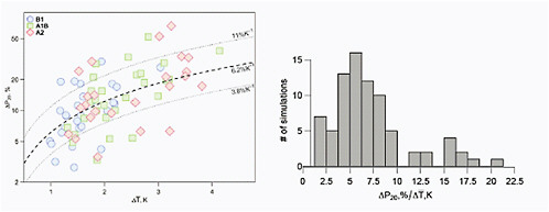
FIGURE 4.10 Relative changes in 20-year return values averaged over the global land area of annual 24-h precipitation maxima (ΔP20) as a function of globally averaged changes in mean surface temperature for B1, A1B, and A2 global emissions scenarios, with results pooled from 14 GCM runs and for 2046-2065 and 2081-2100 relative to 1981-2000. In the left panel, the pooled results are shown along with the median slope of 6.2% per °C and the 15th and 85th percentiles (dashed and dotted lines, respectively). The right panel shows the results as a histogram. Source: Replotted from Kharin et al. (2007, Figure 16).
4.7
SEA ICE, SNOW, AND RELATED FACTORS
Current State of Sea Ice
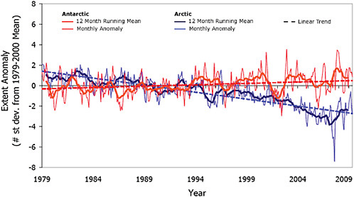
Sea ice plays a critically important role in our climate system. It controls the rate of heat exchange between the polar ocean and atmosphere, reflects much of the solar energy incident on it, helps to maintain the equator-pole temperature gradient, influences ocean circulation, and is of great ecological importance. Typically, sea-ice area is about 14 to 16 million Km2 in late winter in the Arctic and 17 to 20 million Km2 in the Antarctic Southern Ocean. In late summer, on average, only about 3 to 4 million Km2 remain in the Southern Ocean while in the Arctic there are approximately 7 million Km2 (NSIDC; http://nsidc.org/sotc/sea_ice.html). Sea-ice extent, defined here as the area of ocean with at least 15% sea-ice concentration, is negatively correlated to global average surface temperature so that as globally averaged surface temperature increases, sea-ice extent decreases (e.g., Gregory et al., 2002). This sea-ice response to the increasing global surface temperatures occurs directly through thermally driven flux exchanges with the atmosphere and their impact on sea-ice extent and thickness, and indirectly, through the additional impact of increasing temperatures on dynamic mechanisms such as ENSO (e.g., Timmermann et al., 1999) and SAM (e.g., Arblaster and Meehl, 2006). Satellite observations show that there has been a decrease in globally averaged sea-ice extent since 1979. This decrease has occurred in the Arctic, while the Antarctic sea ice has increased slightly (Figure 4.11).
Since the 1950s Arctic sea-ice extent has exhibited a statistically significant decrease (Vinnikov et al., 1999), and the rate of decrease has been faster in summer (–7.8% per decade) than in winter (–1.8% per decade) (Stroeve et al., 2007). Satellite observations beginning in 1978 show that the annual average Arctic sea-ice extent has shrunk by 2.7% per decade (IPCC, 2007a) with larger decreases at the end of summer (9.1% per decade) than at the end of winter (2.9% per decade) (Stroeve et al., 2007). By some measures, from 1979 to 2006, September (late summer) sea-ice extent decreased by almost 25% or about 100,000 km2 per year (Serreze et al., 2007). Comparison of observed Arctic sea-ice decline to IPCC AR4 projections show that the observed rate of ice loss is faster than that predicted by any of the IPCC AR4 models (Stroeve et al., 2007).
The decrease in sea-ice extent has been accompanied by thinning perennial and seasonal ice (Kwok and Rothrock, 2009), a decrease in multiyear ice (Maslanik et al., 2007), and record minima in September sea-ice cover (Serreze et al., 2007; Stroeve et al., 2007; Stroeve et al., 2008). Spring
melt seasons begin earlier and last longer (Serreze et al. (2007). The reduction in sea ice has occurred concurrently with a general increase in surface air temperatures over the Arctic Ocean (Comiso, 2003).
Part of this negative trend in Arctic sea ice has been attributed to natural variability in the atmospheric circulation, which influenced the ice circulation (Rigor and Wallace, 2004), as well as in ocean heat transport from the Atlantic (Polyakov et al., 2005) and the Pacific (Shimada et al., 2006) Oceans. However, natural variability does not account for all of the trend. Part of it has been attributed to increased atmospheric greenhouse gas (GHG) loading. Stroeve et al. (2007) suggest that some 33-38% of the overall observed trend is due to GHG forcing and that for the more recent period 1979-2006 this value may be as high as 47-57%.
Although the whole Arctic has experienced a trend of decreasing sea ice extent, trends in Antarctic sea ice extent have a strong regional signal and have been of opposing sign as demonstrated in Figure 4.12, taken from Liu et al. (2004).
In the Bellingshausen/Amundsen and western Weddell Seas there have
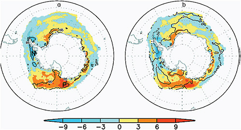
FIGURE 4.12 Spatial trends in Antarctic sea-ice concentration 1979-2002. (a) Trend before removing the influence of AAO and ENSO; (b) Trend after removing the influence of ENSO and the AAO. Source: Liu et al., (2004).
been marked decreases in sea-ice extent, while the Ross Sea has exhibited increasing sea ice extent (Figure 4.12). Due to the opposing regional trends, Antarctic sea-ice extent (Figure 4.11) shows a slight, but statistically significant, positive trend of 0.96±0.61% to 1.0±0.4% per decade, from 1979 to present (Cavalieri and Parkinson, 2008; Turner et al., 2009). This positive trend is led by autumn increases in the Ross Sea followed by the western Pacific Ocean and the Weddell Sea. Recently, the negative trends in the Bellingshausen/Amundsen Seas have decreased, while that in the Indian Ocean has become positive (Cavalieri and Parkinson, 2008). These regional trends in the Antarctic sea ice have been attributed to the influence of atmospheric circulation mechanisms, such asthe SAM (e.g., Thompson and Wallace, 2000), ENSO (e.g., Carleton et al., 1998), and zonal wave three (Raphael, 2007), and stronger cyclonic flow over the Amundsen and Ross Seas associated with stratospheric ozone depletion (Turner et al., 2009). As in the Arctic, there have also been changes in seasonality of the sea ice. The sea-ice maximum appears to occur slightly later in the year, while the sea-ice minimum tends to occur earlier. However, neither trend is statistically significant.
Predictions for Arctic Sea Ice over the 21st Century
The consistent conclusion from all of the model studies is that Arctic sea-ice extent will continue to decrease during the 21st century if emissions of GHGs remain unchecked. This is clearly illustrated in Figure 4.13, which shows the September results from IPCC models using 21st century forcings based on the SRES A1B scenario, a medium-high emissions scenario. In this scenario CO2 concentration is projected to reach 720 ppm by 2100. Although much smaller, the late winter trends are of similar sign. Even with reductions in GHG emissions, Arctic sea-ice extent is predicted to decrease, and the rate of decrease changes with the GHG emission scenario as well as individual model physics. Washington et al. (2009) conducted an analysis of what would occur if CO2 were to be stabilized at 450 ppm at the end of the 21st century. Their results for late summer/early fall (Figure 4.14) show that sea-ice extent for an unmitigated CO2 scenario is reduced by 76% compared to present-day values, whereas for 450 ppm it is reduced only by 24%, preserving 4 million Km2 of sea ice.
Although the predicted year varies, by the end of the 21st century most IPCC models predict an essentially ice-free Arctic (less than 1 million Km2) in late summer. Estimates range from 2037 to 2100 (e.g., Arzel et al., 2006; Boe et al., 2009; Wang and Overland, 2009). The timing depends in part
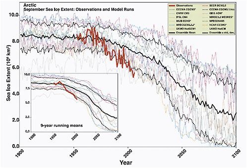
FIGURE 4.13 Arctic September sea-ice extent (× 106 km2) from observations (thick red line) and 13 IPCC AR4 climate models, together with the multi-model ensemble mean (solid black line) and standard deviation (dotted black line). Models with more than one ensemble member are indicated with an asterisk. Inset shows 9-year running means. Source: Stroeve et al. (2007).
on the emission scenario used by the models but may also depend on the natural variability simulated by the individual models. Figure 4.15 taken from Wang and Overland (2009) illustrates this using six IPCC models that simulate the observed mean minimum and seasonality of sea ice very well. Two SRES scenarios are represented: the A1B, which reaches CO2 concentration of 720 ppm by the end of the 21st century, and A2, which reaches 850 ppm at the same time.
The predicted reduction in sea-ice extent is expected to be accompanied by reduction in sea-ice thickness in summer and winter as more areas are replaced by first year ice. Ice in the Northern Hemisphere is expected to thin dramatically as the projected reduction in sea-ice volume is about twice that of the sea-ice extent reduction. Using the same six models in Figure 4.15, Wang and Overland (2009) compare the ice thickness at the time when the
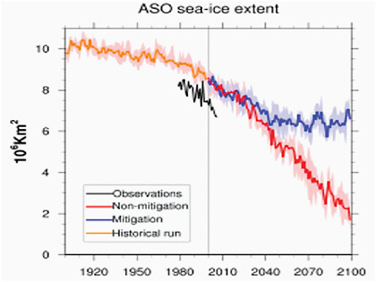
FIGURE 4.14 Time series of August, September and October (ASO) season average Arctic sea ice extent. Dark solid lines are the model ensemble means and the shaded areas show the range of the ensemble members. Observed sea ice is in black. SOURCE: Washington et al., 2009, their Figure 3.
simulated sea-ice extent reaches present-day values (4.6 million km2) in September and March compared to when the sea-ice extent reached nearly ice-free conditions (less than 1.0 million km2) near the end of the 21st century (see Figure 4.16). When sea-ice extent reaches present-day observed values in March much of the central Arctic is covered by sea ice less than 2.5 m thick. By the end of the century this sea ice is less than 2.0 m thick. In September over the same period sea ice moves from being less than 1.2 m thick to nearly ice-free conditions.
The mechanisms involved in reducing sea-ice cover are all positively correlated with temperature increase, giving rise to a linear relationship between annual Arctic sea-ice area reduction and global-averaged surface air temperature. According to one set of estimates, if GHG emissions continue to increase, corresponding temperature increases of 1ºC, 2ºC, 3ºC, and 4ºC are associated with Arctic sea-ice area reductions of 13%, 25%, 36% and 50% respectively (e.g., Gregory et al., 2002: Figure 4). Greater reductions are expected for summer compared to winter. For summer these values are on the order of 24% per degree warming resulting in an ice-free summer
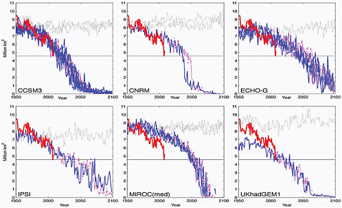
FIGURE 4.15 September sea-ice extent as projected by the six models that simulated the mean minimum and seasonality with less than 20% error of the observations. The colored thin line represents each ensemble member from the same model under A1B (blue solid) and A2 (magenta dashed) emission scenarios, and the thick red line is based on HadISST analysis. Grey lines in each panel indicate the time series from the control runs (without anthropogenic forcing) of the same model in any given 150-year period. The horizontal black line shows the ice extent at 4.6 million km2 value, which is the minimum sea-ice extent reached in September 2007 according to HadISST analysis. All six models show rapid decline in the ice extent and reach ice-free summer (<1 million km2) before the end-of-the-21st-century. Source: Wang and Overland (2009): their Figure 1).
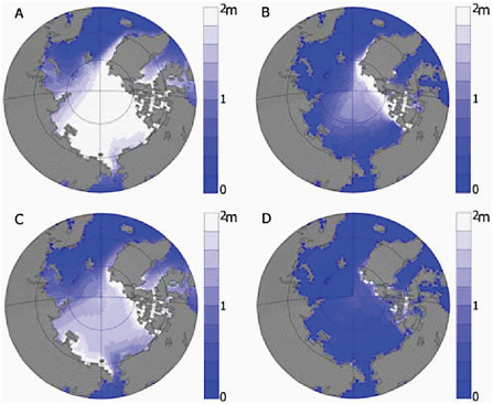
FIGURE 4.16 Mean sea-ice thickness for (left) March and (right) September based on ensemble members from six models under A1B emissions scenario. (a and b) Year when the September ice extent reached 4.6 million km2 by these models and (c and d) year when the Arctic reached nearly sea-ice conditions (less than 1.0 million km2) in September. Source: Wang and Overland, (2009: Figure 3).
by the end of the 21st century for a global warming of 2-4ºC above late 20th century values or 3-5ºC above pre-industrial values This linear relationship between sea-ice loss and global-averaged surface air temperature has implications for sea-ice recovery. One set of simulations using the A1B scenario suggests that Arctic sea ice may recover if GHG emissions were reduced. This response is linear for the annual sea-ice extent but nonlinear for September (Holland et al., 2006, 2010).
Predictions for Antarctic Sea Ice over the 21st Century
Compared to the Arctic very few studies examine the predicted sea-ice changes for the Antarctic. However, many of the characteristics of projected change are like those for the Arctic. Over the 21st century Antarctic sea-ice
cover is projected to decrease. Note that late 20th century and early 21st century observations suggest a slight but significant increase in Antarctic sea-ice extent, contrary to that simulated by the models. This increase is associated with stratospheric ozone depletion and is expected to reverse as ozone returns to normal levels. The predicted decrease will occur more slowly than in the Arctic, particularly in the Ross Sea where temperatures are expected to remain cooler. This is attributed to the fact that the Southern Ocean stores much of its heat increase at depths below 1 km, while in the Arctic Ocean and subpolar seas the heat remains in the upper 1 km (Gregory, 2000; Bitz et al., 2007). In addition, horizontal heat transport poleward of about 60ºN increases in many models (Holland and Bitz, 2003). These differences in the depth where heat is accumulating in the high-latitude oceans influence the relative rates of sea ice decay in the Arctic and Antarctic so that ice loss is faster in the Arctic (IPCC, 2007a).
A comparison of the last 20 years of the 21st century under the SRES A1B scenario with the last 20 years of the 20th century shows a decrease in the sea-ice concentration in both summer (JFM) and winter (JAS) by the end of the 21st century (Meehl et al., 2007; Sen Gupta et al., 2009). (See Figure 4.17.)
IPCC models predict a loss in sea-ice cover in summer and winter ranging from 10-50% in winter, and 33% to total loss in summer by the end of 2100. This is associated with a global warming ranging from 1.7-4.4ºC above late 20th century values. The volume of sea ice is also reduced, and
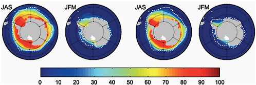
FIGURE 4.17 Multi-model mean sea-ice concentration (%) for January to March (JFM) and June to September (JAS), in the Antarctic for the periods (a) 1980 to 2000 and (b) 2080 to 2100 for the SRES A1B scenario. The dashed white line indicates the present-day 15% average sea-ice concentration limit. Source: Modified from Flato et al. (2004); IPCC (2007a, their Figure 10.14).
this decrease in volume is larger than the decrease in sea-ice concentration, indicating thinning of the sea ice. Substantial sea-ice loss occurs at all longitudes especially in the west Antarctic. In summer the greatest loss is east of the peninsula. Ice loss at these levels suggests a reduction in the seasonal cycle of sea-ice concentration and volume and means a reduction of brine rejection at the margins of Antarctica. This has implications for the future formation of Antarctic deep water and therefore for global ocean heat transport (Sen Gupta et al., 2009).
Snow Cover
Snow cover depends on both temperature and precipitation and is strongly negatively correlated with air temperature. Due to its high albedo, much less solar energy is absorbed by snow-covered areas as contrasted with snow-free areas, and surface temperatures tend to be lower, especially during periods of snow melt. Snow also plays an important role in storing moisture that is released when temperatures rise above freezing. It is a significant variable in the water balance of snow-covered regions and plays an important role in water management, especially in the western United States, where much of the region’s runoff originates in snow that accumulates in mountainous areas in winter. Along with snowfall amounts and snow-covered area, snow water equivalent (SWE) and snow cover duration (SCD) are variables that can be used to characterize snow cover.
Current State of Snow Cover
In the Northern Hemisphere the snow-cover area (SCA) in March has exhibited a negative trend since about 1970, and this decrease has been associated with increased winter temperatures. This correspondence between March SCA and winter temperature appears to have strengthened toward the end of the 20th century (McCabe and Wolock, 2010). Since 1950, SWE has displayed a negative trend in the Pacific Northwest, particularly at lower elevation (Mote, 2003). A shift in the Pacific Decadal Oscillation (PDO) may have contributed to this trend but Mote et al. (2005), in an analysis expanded to include all of the western United States, argued that the PDO alone could not explain the trend in SWE. These conclusions are supported by Hamlet et al. (2005) who attributed the downward trend in SWE to increases in temperature rather than a decrease in precipitation. Figure 4.18 illustrates the observed trends in SWE as well as the trends simulated by the Variable Infiltration Capacity (VIC) hydrologic model. Although some positive trends
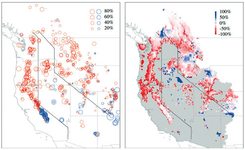
FIGURE 4.18 Linear trends in 1 Apr SWE relative to the starting value for the linear fit (i.e., the 1950 value for the best-fit line): (a) at 824 snow course locations in the western United States and Canada for the period 1950-1957, with negative trends shown by red circles and positive by blue circles; (b) from the simulation by the VIC hydrologic model (domain shown in gray) for the period 1950-1997. Source: Mote et al. (2005: Figure 1).
occurred in, for example, the Southwest, negative trends dominated the region with the largest reductions occurring in western Washington, western Oregon, and northern California.
Accompanying that trend in SWE is a shift in snow melt timing to earlier than average for the contiguous western United States, Alaska, and Canada. Over the period 1966-2007 satellite observations show snow cover reduction over western North America and maritime regions, eastern North America, Scandinavia, and the Pacific coast of Russia (Brown and Mote, 2009).
Predicted Changes in Snow Cover
Snow cover formation and melt are closely related to temperature; therefore snow cover is expected to decrease as temperatures increase. Model results project widespread reductions in snow cover over the 21st century. The Arctic Climate Impact Assessment (ACIA) model mean projects
a reduction in Northern Hemisphere snow cover of 15% by the end of the 21st century under the B2 scenario. Individual, projected reductions range from 9-17%, and are greatest in spring and late summer/early winter, resulting in a shorter snow cover season. The timing of snow accumulation and snow melt is also projected to change. Accumulation is projected to begin later and melt to begin earlier. Fractional snow coverage is also predicted to decrease (Hosaka et al., 2005).
Regionally, the changes are a response to both increased temperature and increased precipitation and are complicated by the competing effects of warming and increased snowfall in those regions that remain below freezing. Taken across models, snow amount and snow coverage decrease in the Northern Hemisphere. Although a number of assessments have been performed of the implications of changes in snow cover on run-off, especially in the western United States (e.g., Hamlet and Lettenmaier, 1999; Christensen et al., 2004; Payne et al., 2004; Christensen and Lettenmaier, 2007), they have mostly been based on off-line simulations wherein hydrology models have been forced with downscaled output from GCMs, rather than as sensitivity analyses, for instance, per degree of global warming. One study that has adopted a sensitivity analysis approach is Casola et al. (2009), which estimated that for each increase in (local, not global) temperature of 1ºC the snowpack should decrease by about 20%. Precipitation changes (precipitation is expected to increase slightly as the climate warms) complicate the snow cover response, which varies with latitude and elevation. When the expected global rate of increase in precipitation was considered, Casola et al. (2009) estimated that the sensitivity of Cascades snowpack would be reduced to 16% per degree C of local warming. Snow amount is projected to increase in other regions, for example, in Siberia. Such increases are thought to be due to increases in precipitation (snowfall) during autumn and winter (Hosaka et al., 2005; Meleshko et al., 2005).
The snow cover variables that are most sensitive to a warming climate are snow cover duration (SCD) and snow water equivalent (SWE). This sensitivity varies with climate regime and elevation, where the largest changes are projected to occur over lower elevations of regions with maritime winter climate, that is, moist climates with snow season temperatures in the range of –5ºC to 5ºC, and the lowest sensitivities are in mid-winter in cold continental climates. In general the models predict an enhanced early response of snow cover to warming over the western cordillera of North America and maritime regions. Over continental interiors, snow cover changes are slower. However, during the 21st century, annual mean SCD is expected to decrease. Although few models show any significant decrease in SCD
during the 20th century, by 2020 the majority of models show significant decrease in SCD over eastern and western North America, Scandinavia, and Kazakhstan. By 2080 the majority of models show significant decreases everywhere. The regions that exhibit the least consensus tend to be continental and that might be due to a slower snow cover change signal. Like SCD, SWE decreases into the 21st century; however, model consensus on the statistical significance of this decrease does not become clear until 2050 when significant decreases occurred over the mid-latitude coastal regions of western Europe and North America (Brown and Mote, 2009).
Permafrost
Permafrost is defined as soil that remains at or below freezing temperatures for two or more years successively. Classified as continuous, discontinuous, and sporadic, permafrost zones occupy about 24% of the Northern Hemisphere exposed land or about 26 million km2 but permafrost underlies only 13-18% of the exposed land (Nelson et al., 1997; Zhang et al., 1999). The active layer of permafrost is the upper layer of soil that thaws in summer and refreezes in winter (Sazonava et al., 2004). In this layer almost all of the below-ground biological processes take place. When it is deep, thawing increases soil moisture storage. Permafrost degradation occurs when temperatures increase in the active layer, and as a result the depth of thaw increases in successive summers and becomes greater than the depth of refreezing.
Although there have been exceptions to the trend (e.g., Brown et al., 2000), in general, observations indicate that the temperature of the permafrost has increased over the 20th century. For example in northern Alaska permafrost temperatures increased by 2 to 7ºC over the 20th century (Lachenbruch and Marshall, 1986; Nelson, 2003). Although the size varies, this warming trend is repeated in northwestern Canada (e.g., Smith et al., 2003), northwestern Siberia (e.g., Pavlov and Moskalenko, 2002), and Scandinavia (Isaksen et al., 2000) among other regions. Along with the higher temperatures, observations show that the active layer is deepening and the permafrost extent is decreasing (Jorgenson et al., 2001; Serreze et al., 2002; Zhang et al., 2005). Since 1900, the maximum area of seasonally frozen ground has decreased by about 7%, led by decreases in spring of up to 15% (Lemke et al., 2007).
Predicted Changes in Permafrost
Climate models predict increases in the depth of thaw over much of the permafrost region. By 2050 seasonal thaw depths are projected to increase by more than 50% in the permafrost regions to the far north including Siberia and northern Canada, while in the southern extents increases of 30-40% are predicted (Stendel and Christensen, 2002; ACIA, 2005; Sasonova et al., 2004). In eastern Siberia permafrost degradation is projected to begin as early as 2050. The increases in thaw depth are associated with warming at the high northern latitudes (e.g., Lawrence and Slater, 2005; Yamaguchi et al., 2005; Kitabata et al., 2006).
The total area covered by continuous, near-surface permafrost (less than 4 m deep) is also projected to decrease and shrink poleward during the 21st century. This is demonstrated in Figure 1 of Stendel and Christiansen (2002), which shows model results for the A2 scenario. Predicted median values for this change are 18, 29, and 41% by 2030, 2050, and 2080 respectively (ACIA, 2005). The size of the decrease varies by model and by warming scenario. For example, Washington et al. (2009) show a range of permafrost loss with the largest losses occurring in their SRES A2 (high emission scenario) and the least in their low emission (450 ppm CO2) scenario. (See Figure 4.19.)
Estimates of near-surface permafrost degradation rates to warming forced by the A1B GHG emissions scenario is on the order of 81,000 km2 per year (Lawrence et al., 2008a). Rates of permafrost degradation may be influenced by rapid Arctic sea ice loss. One climate simulation of such loss predicted warming rates in the western Arctic of 3.5 times greater than the current 21st century climate change trends. This warming signal penetrated inland up to 1,500 km and, although most apparent in autumn, is there year-round. This warming leads to substantial ground heat storage, which in turn degrades the permafrost (Lawrence et al., 2008b).
4.8
SEA LEVEL RISE
The coastal zone has changed profoundly during the 20th century, primarily due to growing populations and increasing urbanization. In 1990, 23 percent of the world’s population (or 1.2 billion people) lived both within a 100 km distance and 100 m elevation of the coast at densities about three times higher than the global average. By 2010, 20 out of 30 mega-cities are on the coast with many low-lying locations threatened by sea level rise. With coastal development continuing at a rapid pace, society is becoming in-
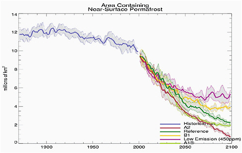
FIGURE 4.19 Time series of model simulations of Northern Hemisphere permafrost up to 2000 and predicted permafrost for several different scenarios after 2000. Dark lines are the model ensemble means and shaded areas show the range of ensemble members. Source: Washington et al. (2009: supplementary figures).
creasingly vulnerable to sea level rise and variability—as Hurricane Katrina recently demonstrated in New Orleans. Rising sea levels will contribute to increased storm surges and flooding, even if hurricane intensities do not increase in response to the warming of the oceans. Rising sea levels will also contribute to the erosion of the world’s sandy beaches, most of which have been retreating over the past century. Low-lying islands are also vulnerable to sea level rise. An increase in global temperature will cause sea level rise and will change the amount and pattern of precipitation, which is important for the stability of ice sheets. The current increase in precipitation over Greenland does not offset the ice loss by melt and fast-flowing glaciers.
Mean, Local, Eustatic, and Steric Sea Level
Mean sea level (MSL) is a measure of the average height of the ocean’s surface (such as the halfway point between the mean high tide and the mean low tide). Local mean sea level (LMSL) is defined as the height of the sea with respect to a land benchmark, averaged over a period of time (such as a month or a year) long enough that fluctuations caused by waves and tides are smoothed out. One must adjust perceived changes in LMSL to account for vertical movements of the land, which can be of the same order (mm y–1) as sea level changes. Some land movements occur because of isostatic adjustment of the mantle to the melting of ice sheets at the end of the last ice age. The weight of the ice sheet depresses the underlying land, and when the ice melts away the land slowly rebounds, whereas some coasts are sinking as a result of isostatic adjustment due to collapsing forebulges in the near-field ocean of previously glaciated regions (Mitrovica and Milne, 2002). Atmospheric pressure, ocean currents and local ocean temperature changes also can affect LMSL. The term eustatic refers to global changes in the sea level brought about by the alteration to the volume of the world ocean (e.g., melting of ice sheets). The term steric refers to global changes in sea level due to thermal expansion and salinity variations. The term isostatic refers to changes in the level of the land masses due to thermal buoyancy or tectonic effects and implies no real change in the volume of water in the oceans.
Global Sea Level
Since 1870, global sea level has risen by about 0.2 m (Bindoff et al., 2007). Since 1993, sea level has been accurately measured globally from satellites. Before that time, the data come from tide gauges at coastal stations around the world. Satellite and tide-gauge measurements show that the rate of sea level rise has accelerated (Figure 4.20). Satellite measurements show sea level is rising at 3.1±0.4 mm y–1 since these records began in 1993 through 2003 (Figure 4.21). This rate has decreased for the most recent time period (2003-2008) to 2.5±0.4 mm y–1 due to a reduction of ocean thermal expansion from 1.6±0.3 mm y–1 to 0.37±0.1 mm y–1, whereas contributions from glaciers, ice caps, and ice sheets increased from 1.2±0.41 mm y–1 to 2.05±0.35 mm y–1, respectively (Cazenave et al., 2008). Statistical analysis reveals that the rate of rise is closely correlated with temperature. Sea level rise is an inevitable consequence of global warming for two main reasons: ocean water expands as it heats up, and additional water flows into the oceans from the ice that melts on land.
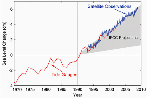
FIGURE 4.20 Sea level change during 1970-2009. The tide gauge data are indicated in red (Church and White, 2006) and satellite data in blue (Cazenave et al., 2008). The grey band shows the projections of the IPCC Third Assessment report for comparison.
Polar Precipitation
Each year, about 8 mm of sea level equivalent accumulates as snow on Greenland and Antarctica. Small changes in precipitation in polar regions will have major affects on the mass balance of the Greenland and Antarctic ice sheets. Increasing temperatures tend to increase evaporation, which leads to more precipitation. Greenland ice sheet precipitation—downscaled from ECMWF operational analyses and re-analyses (Hanna et al., 2005)—follows a significantly increasing trend for 1958-2006. Additional precipitation will occur due to warmer air temperatures mainly in the form of snow accumulation, therefore largely (i.e., ~80%) off sets rising Greenland run-off over the same period (Hanna et al., 2008). The increase in precipitation is confirmed by satellite altimetry data (Johannessen et al., 2005) with a significant growth of 2-5 cm y–1 of the Greenland ice sheet interior from 1992-2004.
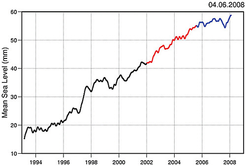
FIGURE 4.21 Sea level curve from Topex/Poseidon and Jason-1 satellite altimetry over 1993-2008 (data averaged over 65ºN and 65ºS; 3-month smoothing applied to the raw 10-day data). Black: Topex/Poseidon; red: Topex/Poseidon plus Jason-1; blue: Jason-1. Source: Cazenave et al. (2008).
The lack of a 20th century trend in net precipitation in recent comprehensive analyses over Antarctica is particularly problematic in the context of 21st century model projections. Almost all climate models simulate a continuing robust precipitation increase over Antarctica in the coming century. During the first half of the 21st century, models using the A1B scenario predict anything from a maximum upward trend of 0.71 mm y–1 to a maximum downward trend of 0.13 mm y–1. Some models project stronger net precipitation increases in the first half of the 21st century, while other models project stronger increases after the middle of the century.
Subsidence
Subsidence is the motion of a surface as it shifts downward relative to a datum such as sea level. Subsidence can be caused by mining, extraction of natural gas, groundwater-related subsidence, isostatic subsidence (change in sedimentation rate), just to name a few, and can locally account for sev-
eral millimeters per year. Some coastal regions are particularly vulnerable to erosion and inundation due to the rapid deterioration of coastal barriers combined with relatively high rates of land subsidence. Subsidence is very important for local sea level assessments and can outweigh the global sea level rate of change on short time scales.
Thermal Expansion
Changes in the climate systems’ energy budget are revealed in ocean temperatures and the associated thermal expansion contribution to sea level rise. Like air and other fluids, water expands as its temperature increases (i.e., its density decreases as temperature increases). As climate change increases ocean temperatures, initially at the surface and over centuries at depth, the water will expand, contributing to sea level rise from thermal expansion. Thermal expansion is likely to have contributed to about 0.025 m of sea level rise during the second half of the 20th century (Meehl et al., 2007), and this rate has increased to about three times during the early 21st century.
The method of calculating average ocean heat content and the associated sea level change using only surface temperatures opens up the possibility of expanding our knowledge into the past and future. Projected rise in global thermosteric sea level for the hypothetical situation where all warming of the sea surface has stopped and the present average temperature is maintained into the future shows that we are committed to a further 0.05 m sea level rise over the next two centuries (Marcčelja, 2009).
Current estimates of thermal expansion account for approximately half of the change observed in global mean sea level rise during the first decade of the satellite altimeter record, but only about a quarter of the change during the previous half century (Figure 4.22). Because this contribution to sea level rise depends mainly on the temperature of the ocean, projecting the increase in ocean temperatures provides an estimate of future growth. Over the 21st century, the IPCC AR4 projected that thermal expansion will lead to sea level rise of about 0.23±0.09 m for the A1B scenario.
Glaciers
Terrestrial glaciers and the Greenland and Antarctic ice sheets have the potential to raise global sea level many meters. Terrestrial glaciers are shrinking all over the world. During the past decade, they have been melting at about twice the rate of the past several decades (Figure 4.22).
Glaciers and mountain ice caps, including those peripheral to Green-
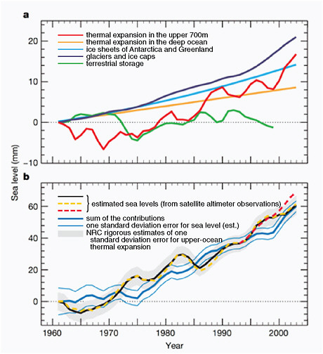
FIGURE 4.22 (a) Total observed sea level rise and its components. The components are thermal expansion in the upper 700 m (red), thermal expansion in the deep ocean (orange), the ice sheets of Antarctica and Greenland (cyan), glaciers and ice caps (dark blue), and terrestrial storage (green). (b), The estimated sea levels are indicated by the black line, the yellow dotted line, and the red dotted line (from satellite altimeter observations). The sum of the contributions is shown by the blue line. Estimates of one standard deviation error for the sea level are indicated by the grey shading. For the sum of components, we include our rigorous estimates of one standard deviation error for upper-ocean thermal expansion; these are shown by the thin blue lines. All time series were smoothed with a 3-year running average and are relative to 1961. Source: Domingues et al. (2008).
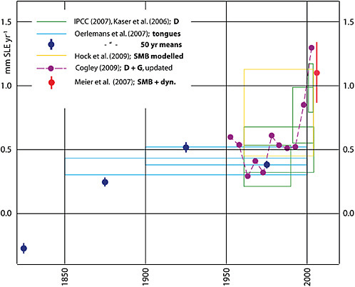
FIGURE 4.23 Estimates of the contribution of glaciers and ice caps to global change in sea level equivalent (SLE), in millimeters SLE per year. Source: Allison et al. (2009b).
land and Antarctica, can potentially contribute a total of approximately 0.7 m to global sea level, and they provide a source of freshwater in many mountain regions worldwide (Bahr et al., 2009). For 1961-2003, glaciers and ice caps contributed 0.5±0.2 mm y–1 to global sea-level rise (Figure 4.22), increasing to 0.8±0.17 mm y–1 for 1993-2003 (Allison et al., 2009b). This new assessment (Figure 4.23) shows ice loss from glaciers and ice caps slightly higher than those reported in IPCC AR4, contributing now about 1.2±0.2 mm y–1 to global sea level rise. Glaciers and ice caps are not in balance with the present climate; glaciers need to decrease in volume by 27% on average, and ice caps need to decrease by 26% to attain equilibrium
(Bahr et al., 2009). A future equilibrium with the current climate implies a change in sea level of 0.089±0.015 m due to glaciers and 0.095±0.029 m due to ice caps, with a total change in sea level of 0.184±0.033 m.
The ratio of accumulation area (AAR) at the end of the melt season and total glacier area dropped from roughly 0.54 in 1961 to 0.44 in 2007, and it is expected to drop further to 0.31 by 2050. This is a conservative estimate—observations indicate a faster than linear decrease in global ice mass balance over the past 40 years (Kaser et al., 2006). Although the actual decrease in AAR may be faster than linear, this conservative estimate represents a 30% decrease from the current value. As a rough approximation, we can assume that the AAR of every glacier decreases by the same percentage, giving an estimate of the fractional volume change for each glacier. In that case, the minimal sea level rise from glaciers and ice caps will be 0.373±0.021 m over the next 100 years (Bahr et al., 2009).
Greenland and Antarctic Ice Sheets
On the polar ice sheets, there is observational evidence of accelerating flow from outlet glaciers both in Greenland and in west Antarctica. Both inland snow accumulation and marginal ice melting have increased over the Greenland ice sheet, but there is little evidence for any significant accumulation trend over the Antarctic ice sheet. Antarctica and Greenland maintain the largest ice reservoirs on land. For 1993-2003, the estimated contributions for the Greenland and Antarctic ice sheets are 0.21±0.07 mm y–1 and 0.21±0.35 mm y–1, respectively (Bindoff et al., 2007). There is little information to constrain ice sheet contributions for previous decades, but it is thought that the Greenland contribution has increased significantly in recent years (Lemke et al., 2007). Since IPCC AR4, there have been a number of new studies on ice sheet mass budget that have considerably enhanced our understanding of ice sheet vulnerabilities (Figure 4.24) (Allison et al., 2009a). Recent observations have shown that changes in the rate of ice discharge into the sea can occur far more rapidly than previously suspected (e.g., Rignot, 2006).
The pattern of ice sheet change in Greenland is one of near-coastal thinning, primarily along fast-moving outlet glaciers. Accelerated flow and discharge from some major outlet glaciers (also called dynamic thinning) is responsible for much of the loss (Rignot and Kanagaratnam, 2006; Howat et al., 2007). Pritchard et al. (2009) used high-resolution satellite laser altimetry to show that dynamic thinning of fast-flowing coastal glaciers is now widespread at all latitudes in Greenland. Figure 4.24 shows estimates
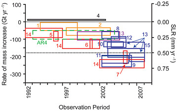
FIGURE 4.24 Estimates of the net mass budget of the Greenland Ice Sheet since 1992 (Allison et al., 2009b). The horizontal dimension of the boxes shows the time period for which the estimate was made, and the vertical dimension shows the upper and lower limits of the estimate. The colors represent the different methods that were used: black is satellite radar altimetry, orange is aircraft laser altimetry, purple is aircraft/satellite laser altimetry, red is the flux component method, and blue is satellite gravity.
of the mass balance of the Greenland ice sheet that have been made since the early 1990s. The horizontal dimension of the boxes shows the time period for which the estimate was made, and the vertical dimension shows the upper and lower limits of the estimate. The colors represent the different methods that were used: black is satellite radar altimetry, orange is aircraft laser altimetry, purple is aircraft/satellite laser altimetry, red is the flux component method, and blue is satellite gravity. The dashed green box represents the estimated Greenland balance of the IPCC AR4 assessment. These data indicate that mass loss from the Greenland ice sheet may be increasing, although it is also clear that the various estimates are frequently not in agreement. Greenland lost roughly 150 Gt y–1 since 2000, increasing to 180±50 Gt y–1 (0.5±0.14 mm y–1 SLR) for the time period 2003-2007. More than 50% of the current ice loss is caused by increase in ice discharge and ocean interaction of tidewater glaciers, the remaining part can be explained by the increase in surface melt due to warmer summer temperatures (Hanna et al., 2008). The interior of the ice sheet is expected to be less vulnerable to future changes than the edge regions. Current discharge rates may represent a transient instability, and whether they will increase or decrease in the
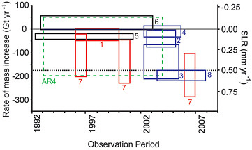
FIGURE 4.25 Estimates of the net mass balance of the Antarctic Ice Sheet since 1992 (Allison et al., 2009b). The horizontal dimension of the boxes shows the time period for which the estimate was made, and the vertical dimension shows the upper and lower limits of the estimate. The colors represent the different methods that were used: black is satellite radar altimetry, orange is aircraft laser altimetry, red is the flux component method, and blue is satellite gravity.
future is unknown. Currently there is no dynamic ice sheet model that can predict the response of the Greenland ice sheet for a warmer climate. We can constrain a possible upper bound of SLR contribution from Greenland assuming a doubling in ice discharge and a continued increase in surface melt using the AR4 A1B scenario (Pfeffer et al., 2008). The total contribution to SLR would be about 0.16 m by 2100, with 0.09 m contribution from ice dynamics, and 0.07 m from surface melt (Pfeffer et al., 2008).
The Antarctic ice sheet shows a pattern of near balance for East Antarctica and mass loss from West Antarctica and the Antarctic Peninsula since 2003 (Cazenave et al., 2009). However, the uncertainties of these measurements are large (Figure 4.25) and there is no strong evidence for increasing Antarctic loss over the period shown.
However, there is a region in West Antarctica that shows increasing ice loss in recent years (Figure 4.25, most of this signal comes from West Antarctica). The Amundsen Coast Basin, including Pine Island ice and Thwaites Glacier, is not confined by large ice shelves, and these marine-based ice masses, which are potentially unstable, contain about 1.5 m sea level equivalent. The average ice velocity in this region is 2 km y–1, which is considerably higher than the average velocity of all Antarctic ice streams (0.65 km y–1) (Pfeffer et al., 2008). If this ice discharge continues to increase, SLR contribution from West Antarctica cannot be ignored. Pfeffer
et al. (2008) assume in their sea level rise sensitivity study for Antarctica a doubling of outlet glacier velocities in Pine Island and Thwaites Glacier within the first decade, and ice loss acceleration from the Antarctic Peninsula at the same rate than melt increase at present-day rates of surface mass balance change, resulting in a sea level rise of 0.12 m by 2100, just from the increase in ice discharge.
Summary of Sea Level Change
Greenland and Antarctic ice sheets together would contribute up to 0.285 m sea level under the AR4 A1B warming scenario, assuming a doubling in ice discharge for the Greenland outlet glaciers, and the Amundsen Coast Basin in Antarctica. Such an increase in ice discharge has already been observed for several regions in Greenland. Glaciers and ice caps are expected to contribute 0.37±0.02 m sea level rise under the same warming scenario, and thermal expansion is expected to contribute 0.23±0.09 m by 2100.
Thus, the sea level rise by 2100 is expected to be at least 0.60±0.11 m from thermal expansion and ice loss from glaciers and small ice caps only. Assuming additional ice loss from Greenland at the rate, the total global sea level rise would be about 0.65±0.12 m by 2100. Doubling in ice discharge for both Greenland and Antarctica, the sea level increase could be as high as about 0.88 ±0.12m by 2100. The estimated range in sea level rise in 2100 is therefore from about 0.5 to 1 m.
The dynamic response of ice sheets to global warming is the largest unknown in the projections of sea level rise over the next century. Vermeer and Rahmstorf (2009) made a semi-empirical projection linking sea level to temperatures from past observations; their statistical projection for a temperature scenario A1B (IPCC AR4: 2.3-4.3ºC increase for 2100) predicts a SLR of 0.97-1.56 m above 1990 by 2100. This is consistent with what happened during warming in the last interglacial time period (LIG) and cannot be ruled out. The LIG warming was caused by perturbations of Earth’s orbit (Overpeck et al., 2006) and arrived much more gradually than is projected for human-induced warming, so a faster sea level rise in the future than in the LIG would not be surprising. On the other hand, changes in the LIG were linked to ice at low elevation, which could behave differently from that at high elevation in the interior of Greenland.
4.9
OCEAN ACIDIFICATION
The oceanic uptake of excess atmospheric carbon dioxide alters the chemistry of seawater, which may impact a wide range of marine organisms from plankton to coral reefs (Doney et al., 2009a,b; NRC, 2010) (see also Section 6.3). Ocean acidification is in fact a series of interlinked and wellknown changes in acid-base chemistry and carbonate chemistry due to the net flux of CO2 into surface waters (Figure 4.26). The chemical shifts include increases in the partial pressure of carbon dioxide (pCO2), the concentration of aqueous CO2, and the hydrogen ion (H+) concentration and decreases in pH (pH = –log10[H+]). The increase in hydrogen ion concentration acts to lower the concentration of carbonate ions (CO32–) through the reaction H+ + CO32– => HCO3–, even though the total amount of dissolved inorganic carbon (DIC) goes up (DIC = [CO2] + [HCO3–] + [CO32–]). Declining CO32– in turn lowers calcium carbonate (CaCO3) mineral saturation state, Ω = [Ca2+][CO32–]/Ksp, where Ksp is the thermodynamic solubility product that varies with temperature, pressure, and mineral form. Ocean surface waters
![FIGURE 4.26 Schematic indicating the effects on seawater carbonate chemistry due to the uptake of excess carbon dioxide (CO2) from the atmosphere. Ocean acidification causes increases in some chemical species (red) and decreases in other species (blue). Ocean acidification also causes a reduction in pH (pH = –log10[H+]) and the saturation states, Ω, of calcium carbonate minerals in shells and skeletons of planktonic and benthic organisms and in carbonate sediments. On millennial and longer time scales, ocean pH perturbations are buffered by external inputs of alkalinity, denoted by calcium ions (Ca2+) and changes in the net burial rate of carbonate sediments.](/openbook/12877/xhtml/images/p2001cde0g154001.jpg)
FIGURE 4.26 Schematic indicating the effects on seawater carbonate chemistry due to the uptake of excess carbon dioxide (CO2) from the atmosphere. Ocean acidification causes increases in some chemical species (red) and decreases in other species (blue). Ocean acidification also causes a reduction in pH (pH = –log10[H+]) and the saturation states, Ω, of calcium carbonate minerals in shells and skeletons of planktonic and benthic organisms and in carbonate sediments. On millennial and longer time scales, ocean pH perturbations are buffered by external inputs of alkalinity, denoted by calcium ions (Ca2+) and changes in the net burial rate of carbonate sediments.
are currently supersaturated (Ω> 1) for the two major forms used by marine organisms, aragonite (corals, many mollusks) and calcite (coccolithophores, foramaniferia, and some mollusks,). Because of pressure effects and higher metabolic CO2 from organic matter respiration, Ω decreases with depth often becoming undersaturated (Ω< 1), at which point unprotected shells and skeletons begin to dissolve.
The controls on seawater pH and saturation state vary with time-scale. In the surface ocean, the pH of seawater varies substantially over annual to interannual time scales due to the net biological formation of organic matter (lowers CO2 and raises pH and Ω) and CaCO3 shells and skeletons (the reverse). Upwelling of CO2-rich water from below and variations in temperature, salinity, and alkalinity (a measure of the acid buffering capacity of seawater) also influence surface water carbonate chemistry. The saturation state of polar waters is lower in large parts because of colder temperatures. In coastal waters, pH and Ω exhibit large natural spatial and temporal variations due to the interplay of river runoff, strong biological productivity, and in, some locations, coastal upwelling (Salisbury et al., 2008). Over decadal to century time scales, ocean carbon chemistry is modulated by net CO2 uptake from the atmosphere and trends in ocean circulation and biological productivity, which tend to redistribute dissolved inorganic carbon and alkalinity within the ocean water-column. On even longer time scales of many centuries to millennia, the weathering of calcium carbonate rocks on land adds alkalinity, a measure of the acid buffering capacity, in the form of calcium ions (Ca2+) and carbonate ions (CO32–), and alkalinity is removed by the burial, on continental shelves and margins, of biologically formed carbonate sediments made of the shells and skeletons of some plankton, corals, and other calcifying organisms (Figure 4.26). Carbonate sediment burial rates are sensitive to seawater chemistry, and on millennial time scales longer, efficient damping feedbacks act to stabilize mean ocean alkalinity and pH.
At the small number of available open-ocean time-series sites, significant secular trends in surface ocean carbonate chemistry are well documented for the past two decades (Figure 4.27). The time-series records document clearly an increase in surface water pCO2 and DIC and a decline in pH that is consistent with the rate of change in atmospheric CO2 (Dore et al., 2009). The WOCE/JGOFS Global CO2 Survey completed in the 1990s provided a global estimate of ocean anthropogenic CO2 distributions and a baseline for assessing changes in ocean chemistry with time (Sabine et al., 2004). Decadal resurveys of a subset of the WOCE/JGOFS ocean transects also exhibit decreasing pH through time over the upper thermocline and
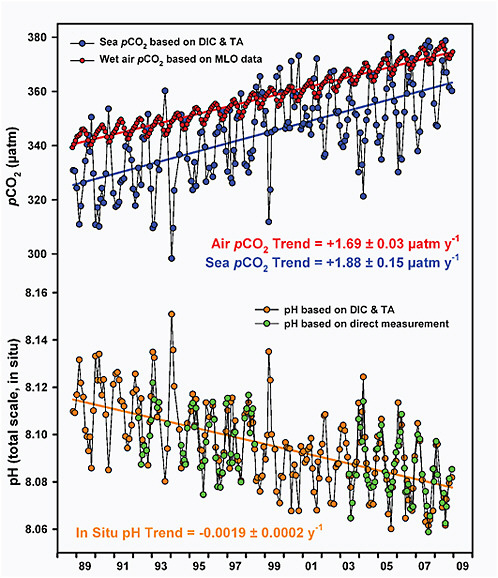
FIGURE 4.27 Time-series surface seawater carbonate system at Station ALOHA in the subtropical North Pacific north of Hawai’i, 1988-2008. The upper panel displays the partial pressure of CO2 (pCO2) in seawater calculated from dissolved inorganic carbon (DIC) and total alkalinity (TA) (blue symbols) and in water-saturated air at in-situ seawater temperature (red symbols). Atmospheric CO2 data is from the Mauna Loa Observatory, Hawai’i. The lower panel displays in-situ surface pH based on direct measurements (green symbols) or as calculated from dissolved inorganic carbon and total alkalinity (orange symbols). Linear regressions (colored lines) and regression equations are reported for each variable. Source: Adapted from Dore et al. (2009).
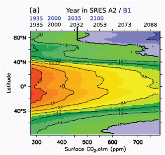
FIGURE 4.28 Projected evolution of the annual-mean, zonally averaged aragonite saturation, Ω, plotted as a function of the annual-mean atmospheric CO2 mixing ratio at the ocean surface. The corresponding years for the SRES A2 and B1 scenarios are given at the top. The largest decreases in aragonite saturation values occur in the tropics. Arctic and Southern Ocean surface waters transition from supersaturation to undersaturation in the annual-mean beginning at approximately 460 ppm and 550 ppm CO2, respectively. Undersaturated conditions occur for individual months at even lower atmospheric CO2 levels, beginning at approximately 410 ppm for the Arctic and 490 ppm for Southern Ocean. Source: Adapted from Steinacher et al. (2009).
across ocean basins (Byrne et al., 2010). Based on ice-core CO2 data and the WOCE/JGOFS Survey, surface ocean pH has already dropped on average by about 0.1 pH units from pre-industrial levels (pH is measured on a logarithmic scale and a 0.1 pH drop is equivalent to a 26% increase in hydrogen ion concentration) (Orr et al., 2005). The patterns of ocean acidification in subsurface waters depend on ocean circulation patterns; thermocline waters in subtropical convergence regions and deep-waters in polar regions where cold surface waters sink into the interior ocean are affected more than other parts of the subsurface.
Future acidification of surface waters can be predicted for a given atmospheric carbon dioxide level (see Figure 4.28). An additional decline of 0.15 pH unit would occur if atmospheric carbon dioxide increases from current levels to 550 ppm, and larger pH changes would occur, approximately
proportionally, for higher CO2 concentrations. Polar surface waters may become under-saturated with respect to aragonite, a key calcium carbon mineral that can affect the ability of organisms to build their shells, for atmospheric CO2 levels of 400-450 ppm for the Arctic and 550-600 ppm for the Antarctic (Orr et al., 2005; Steinacher et al., 2010). For tropical surface waters, large reductions in calcium carbonate saturation state are expected to occur, but waters are expected to remain super-saturated for projected atmospheric CO2 during the 21st century for current scenario projections. Calcium saturation horizons (Ω = 1) have been observed to move upward, that is, shoaled (Feely et al., 2004; Orr et al., 2005), and there is evidence that water undersaturated for aragonite is already upwelling onto the continental shelf off the U.S. west coast due to a combination of strong wind-induced upwelling and the penetration of anthropogenic CO2 into off-shore source waters (Feely et al., 2008). For most of the surface ocean, climate change feedbacks are weak, and warming and altered ocean circulation have a limited effect on changing pH and Ω that are determined primarily by atmospheric CO2. An exception is in the Arctic, where sea-ice retreat and changes in surface freshwater balance amplify atmospheric CO2-driven pH and Ω declines (Steinacher et al., 2010).


