
2
Emissions, Concentrations, and Related Factors
2.1
CONTRIBUTION OF DIFFERENT CHEMICALS TO CO2EQUIVALENT LEVELS AND CLIMATE CHANGES
A range of anthropogenic chemical compounds contribute to changing Earth’s energy budget, thereby causing the planet’s global climate to change. For example, increases in greenhouse gases absorb infrared energy that would otherwise escape to space, acting to warm the planet, while some types of aerosol particles can contribute to cooling the planet by reflecting incoming visible light from the Sun. These components of our atmosphere are emitted from a variety of human activities, including for example fossil fuel burning, land-use change, industrial processes such as cement production, and agriculture. The gases and particles involved are frequently referred to as drivers of climate change, or radiative forcing agents. Detailed reviews of radiative forcing is presented in Forster et al. (2007) and Denman et al. (2007). Radiative forcing due to various climate change agents can be converted to equivalency with the concentration of CO2 (CO2 equivalent), one frame of reference for this report (see Figure 2.1). Here we briefly summarize how major forcing agents contribute to current and future CO2-equivalent target levels and explore implications for global mean temperature increases.
Some greenhouse gases and aerosols are retained for days to years in the atmosphere after emission. The concentrations of such compounds in the atmosphere are tightly coupled to the rate of emission. Their concentrations would drop rapidly if emissions were to cease. Increasing emissions lead to increases in concentrations of such gases, while constant emissions are required for their concentrations to be stabilized. Methane is a key greenhouse gas with an atmospheric lifetime of about 10 years whose concentration has approximately doubled since the pre-industrial era (1750), and it is the second most important greenhouse gas, currently contributing about
25 ppmv of CO2 equivalent (see Figure 2.1). From about 1998 to 2007, methane concentrations remained nearly constant (Forster et al., 2007). However, methane began to increase after 2007. In the absence of mitigation, methane is expected to continue to make significant contributions to climate change during the 21st century (see Section 2.2).
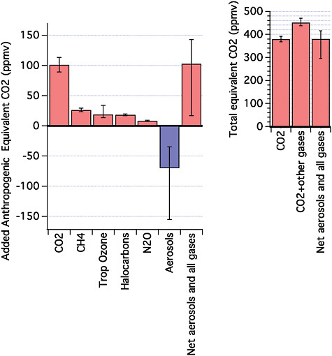
FIGURE 2.1 (left) Best estimates and very likely uncertainty ranges for aerosols and gas contributions to CO2-equivalent concentrations for 2005, based on the radiative forcing given in Forster et al. (2007). All major gases contributing more than 0.15 W m–2 are shown. Halocarbons including chlorofluorocarbons, hydrochlorofluorocarbons, hydrofluorocarbons, and perfluorocarbons have been grouped. Direct effects of all aerosols have been grouped together with their indirect effects on clouds. (right) Total CO2-equivalent concentrations in 2005 for CO2 only, for CO2 plus all gases, and for CO2 plus gases plus aerosols.
In sharp contrast, some greenhouse gases have biogeochemical properties that lead to atmospheric retention times (lifetimes) of centuries or even millennia. These gases can accumulate in the atmosphere whenever emissions exceed the slow rate of their loss, and concentrations would remain elevated (and influence climate) for time scales of many years even in the complete absence of further emission. Like the water in a bathtub, concentrations of carbon dioxide are building up because the anthropogenic source substantially exceeds the natural net sink. Even if human emissions were to be kept constant at current levels, concentrations would still increase, just as the water in a bathtub does when the water comes in faster than it can flow out the drain. The removal of anthropogenic carbon dioxide from the atmosphere involves multiple loss mechanisms, spanning the biosphere and ocean (see Section 2.4), and carbon dioxide removal cannot be characterized by any single lifetime. Although some carbon dioxide would be lost rapidly to the terrestrial biosphere and to the shallow ocean if human emissions cease, some of the enhanced anthropogenic carbon will remain in the atmosphere for more than 1,000 years, influencing global climate (Archer and Brovkin, 2008). The warming induced by added carbon dioxide is expected to be nearly irreversible for at least 1,000 years (Matthews and Caldeira, 2008; Solomon et al., 2009), see Section 3.4.
Figure 2.1 shows that carbon dioxide is the largest driver of current anthropogenic climate change. Other gases such as methane, nitrous oxide, and halocarbons also make significant contributions to the current total CO2-equivalent concentration, while aerosols (see Section 2.3) exert an important cooling effect that offsets some of the warming. The best estimate of net total CO2 equivalent concentration of the sum across these forcing agents in the year 2005 is about 390 ppmv (with a very likely range from 305 to 430 ppmv). Global carbon dioxide emissions have been increasing at a rate of several percent per year (Raupach et al., 2007). If there were to be no efforts to mitigate its emission growth rate, scenario studies suggest that carbon dioxide could top 1,000 ppmv by the end of the 21st century. Carbon dioxide alone accounts for about 55% of the current total CO2-equivalent concentration of the sum of all greenhouse gases, and it will increase to between 75 and 85% by the end of this century based on a range of future emission scenarios (see Section 2.2). Thus carbon dioxide is the main forcing agent in all of the stabilization targets discussed here, but the contributions of other gases and aerosols to the total CO2-equivalent remain significant, motivating their consideration in analysis of stabilization issues.
How large a reduction of emissions is required to stabilize carbon dioxide concentrations, and does it depend upon when it is done or on the
chosen target stabilization concentration? Studies over the past five years of so using many different carbon cycle models have improved our understanding of requirements for carbon dioxide stabilization. This is because of more detailed treatments of carbon-climate feedbacks, including the ways in which warming decreases the efficiency of carbon sinks as compared to earlier work (e.g., Jones et al., 2006; Matthews, 2006). Figure 2.2 shows an example of stabilization for two different Earth Models of Intermediate Complexity (EMICs), the University of Victoria (UVIC) model and the Bern model (see Methods section for descriptions of these two models; see also Plattner et al., 2008, and references therein for a model intercomparison study). In this example test case, carbon dioxide emissions increase at current growth rates of about 2% per year to a maximum of about 12 GtC per
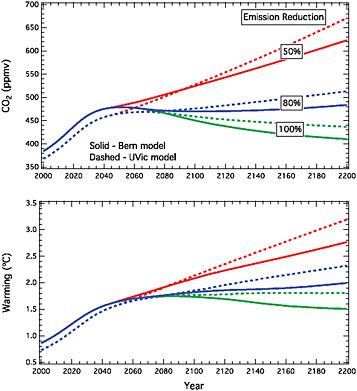
FIGURE 2.2 Illustrative calculations showing CO2 concentrations and related warming in two EMICS (the Bern model and the University of Victoria model, see Methods) for a test case in which emissions first increase, followed by a decrease in emission rate of 3% per year to a value 50%, 80%, or 100% below the peak. The test case with 100% emission reduction has 1 trillion tonnes of total emission and is also discussed in Section 3.4.
year, followed by a decrease of 3% per year down to a selected total reduction of 50, 80, or 100%. The rate of decrease of 3% per year used here is derived from scenario analysis described in the next section. This section together with the next section aim to probe what plausible rates of emissions reduction based upon scenario studies imply for the future evolution of carbon dioxide concentrations. The rate of possible emissions reductions of carbon dioxide depends upon factors including e.g., commitments to existing infrastructure and development of alternatives, see Section 2.2. It is interesting to note that even in the case of the phaseout of ozone-depleting substances under the Montreal Protocol, emissions reductions were about 10% per year initially but stalled at a total reduction of about 80% of the peak, with some continuing emissions of certain gases occurring due for example, the challenge of finding alternatives for fire-fighting applications (see IPCC, 2005).
Figure 2.2 shows that carbon emission reductions of 50% do not lead to long-term stabilization of carbon dioxide, nor of climate, in either of these models, as has also been shown in previous studies (e.g., Weaver et al., 2007). It is noteworthy that the Bern model has weaker carbon-climate feedbacks than the UVIC model; nevertheless both models show the need for emissions reductions of at least 80% for carbon dioxide stabilization even for a few decades, while longer-term stabilization requires nearly 100% reduction. Very similar results were obtained in other test cases run for this study considering peaking at higher values, or decreasing at rates from 1 to 4% per year (see also Meehl et al., 2007; Weaver et al., 2007). Figure 2.3 shows sample calculations evaluated in Meehl et al. (2007) using three different models for various stabilization levels. Figure 2.3 shows that stabilization levels of 450, 550, 750, or 1,000 ppmv require eventual emission reductions of 80% or more (relative to whatever peak emission occurs) in all of the models evaluated. Thus current representations of the carbon cycle and carbon-climate feedbacks show that anthropogenic emissions must approach zero eventually if carbon dioxide concentrations are to be stabilized in the long term (Matthews and Caldeira, 2008). This is a fundamental physical property of the carbon cycle and is independent of the emission pathway or selected carbon dioxide stabilization target. Box 2.1 discusses how emissions of non-CO2 greenhouse gases could affect attainment of stabilization targets.
Figures 2.2 and 2.3 illustrate a fundamental change in understanding stabilization of climate change that has been prompted by the scientific literature of the past two years or so (see Jones et al., 2006; Matthews and Caldeira, 2008). Early work on stabilization using relatively simple models
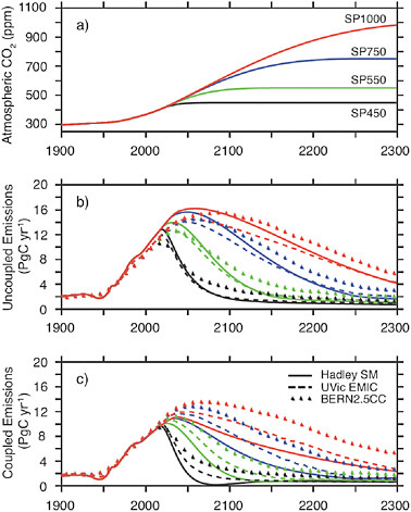
FIGURE 2.3 (a) Illustrative atmospheric CO2 stabilization scenarios for 1,000, 750, 550, and 450 ppmv; SP1000 (red), SP750 (blue), SP550 (green) and SP450 (black), from Meehl et al. (2007). (b) Compatible annual emissions calculated by three models, the Hadley simple model (solid), the UVIC EMIC (dashed), and the BERN2.5CC EMIC (triangles) for the three stabilization scenarios. Panel (b) shows emissions required for stabilization without accounting for the impact of climate on the carbon cycle, while panel (c) included the climate impact on the carbon cycle, showing that emission reductions in excess of 80% (relative to peak values) are required for stabilization of carbon dioxide concentrations at any of these target concentrations.
suggested that slow reductions in emissions could lead to eventual stabilization of climate (e.g., Wigley et al., 1996). But recent studies using more detailed models of key feedbacks in the ocean, biosphere, and cryosphere, have underscored that although a quasi-equilibrium may be reached for a limited time in some models for some scenarios, stabilizing radiative forcing at a given concentration does not lead to a stable climate in the long run. Cumulative emitted carbon can more readily be linked to climate stabiliza-
|
BOX 2.1 STABILIZATION AND NON-CO2GREENHOUSE GASES Because carbon emissions reductions of more than 80% are required to stabilize carbon dioxide concentrations, small continuing emissions of carbon dioxide, or emissions of CO2-equivalent through other gases, could have surprisingly important implications for stabilizing climate change. For example, emissions of the hydrofluorocarbons (HFCs) currently used as substitutes for chlorofluorocarbons make a small contribution to today’s climate change. However, because emissions of these gases are expected to grow in the future if they are not mitigated, and because of the stringency of the requirement of near zero emissions of CO2-equivalent, these gases could represent a significant future impediment to stabilization efforts. For example, Figure 2.4 below shows that in the absence of mitigation, the HFCs could represent as much as one-third of the allowable CO2-equivalent emissions in 2050 required for a stabilization target of 450 CO2-equivalent. Thus, the analysis presented here underscores that stabilization of climate change requires consideration of the full range of greenhouse gases and aerosols, and of the full suite of emitting sectors, applications, and nations. 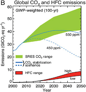 FIGURE 2.4 Global CO2 and HFC emissions expressed as CO2-equivalent emissions per year for the period 2000-2050. The emissions of individual HFCs are multiplied by their respective GWPs (direct, 100-year time horizon) to obtain aggregate emissions across all HFCs expressed as equivalent GtCO2 per year. High and low estimated ranges based on analysis of likely demand for these gases and assuming no mitigation of HFCs are shown. HFC emissions are compared to emissions for the range of SRES CO2 scenarios, and two 450-and 550-ppm CO2 stabilization scenarios. The estimated CO2-equivalent emissions due to HFCs in the absence of mitigation reach about 6 GtCO2-equivalent in 2050, or about a third of the emissions due to CO2 itself at that time in the 450 ppm stabilization scenario. Source: Velders et al. (2009). |
tion, due to the irreversible character of the induced warming driven by carbon dioxide (see Section 3.4).
2.2
INFORMATION FROM SCENARIOS
Figure 2.5 shows the emissions of manmade greenhouse gases from various sectors of the U.S. economy (U.S. EPA, 2008). For highly industri-
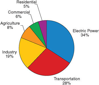
FIGURE 2.5 U.S. greenhouse gas emissions by sector in 2006. Source: U.S. EPA (2008).
alized countries such as the United States, the difficulty in reducing emissions will depend in large part on the lifetimes of the existing capital stock associated with the major emitting sectors. The electric sector is the largest source of manmade emissions in the United States, primarily due to the carbon dioxide emitted during the combustion of fossil fuels. The lifetime of coal-fired power plants is measured in decades. The next largest source of U. S. greenhouse gases is the transportation sector, again due to the combustion of fossil fuels. Here the lifetime of the capital stock is typically a decade or two.
Although developed countries historically have been the major emitter of greenhouse gases, developing countries are on track to overtake them in the next few years. In their case, the issue becomes one of the capital stock put in place in the future to support their industrialization process. With the huge economic growth projected for developing countries and in the absence of incentives to act otherwise, these countries will likely turn to the cheapest energy sources to fuel their growth. These fuels currently are fossil based: coal, oil, and gas. A recent study by the Energy Modeling Forum, based on eight Energy-Economy models, projected an annual growth rate of CO2 emissions globally from the burning of fossil fuels and industrial uses to be of the order of 1 to 2 percent per year over the remainder of the
century, in the absence of intervention (EMF 22, 2009). The study attributes much of the growth to developing countries.
Even if wealthier countries like the United States were to reduce their emissions to zero immediately, it is unlikely that global CO2 emissions would be stabilized, much less global atmospheric concentrations (Blanford et al., 2009). Being in their post-industrial phase of development, the economic growth rates in developed countries are expected to be lower than those of developing countries and their mix of goods and services less carbon intensive. The cumulative reductions of developed countries, even with aggressive emissions reduction programs, are expected to be low when compared to those of developing countries.
One important contribution that developed countries can make to global emissions reductions is to develop the technological wherewithal that would not only be necessary for their own emission reductions, but also would be essential for developing countries to meet their economic development goals with affordable climate-friendly technologies.
As noted above, both the existing capital stock and that put in place in the future are critical to understanding the difficulty of transitioning away from the current path of growth in greenhouse gas emissions. Figure 2.6 shows representative carbon pathways (RCPs) for limiting radiative forcing (watts per m2) at two alternative levels. These are referred to as the RCP 2.61 and RCP 4.5 scenarios. These are among a suite of pathways being developed for use in the IPCC 5th Assessment. The pathways shown in the figure were developed by the IMAGE and MiniCAM models, respectively (Moss et al., 2010).
Figure 2.6 highlights the importance of the carbon budget, that is, the area under the allowable emissions curve associated with a particular radiative forcing target. Being much lower in the RCP 2.6 scenario than in the RCP 4.5 scenario, we see the rate of growth first slows and then rapidly decline beginning in 2020. In the case of the higher CO2 budget, emissions rise for another two decades before peaking. Notice that the maximum rate of decline is comparable in the two scenarios (about 3.5% per year); however, in the latter it is shifted out in time. The reasons for this shift are both the higher
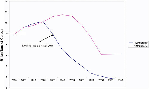
FIGURE 2.6 shows representative carbon pathways (RCPs) for limiting radiative forcing (W per m2) at two alternative levels. The tighter the limit, the earlier the reductions must take effect. With the RCP 2.6 scenario, the rate of growth first slows and then rapidly declines beginning in 2020. In the case of the less stringent constraint, emissions rise for another two decades before peaking. Here the decline is shifted out in time.
carbon budget and a greater array of low-carbon, economically competitive alternatives, which are assumed to become available in the future.
We stress that there is a great deal of flexibility regarding the rate at which new technologies are substituted for existing ones, both on the supply and demand sides of the energy sector. The rate of retirement of existing carbon-intensive plant and equipment and their replacement with more climate-friendly alternatives will depend upon a number of factors. These include the stabilization target, reference case emissions in the absence of a price on CO2 (either explicit or implicit), the availability and costs of alternatives, and the willingness to pay the costs of the transition to a low-carbon economy. The latter will depend on society’s perception of the benefits (reduction in damages due to climate change). From a purely physical perspective, decline rates much higher than those shown here are feasible. It is a matter of the perceived urgency and the motivation to decarbonize.
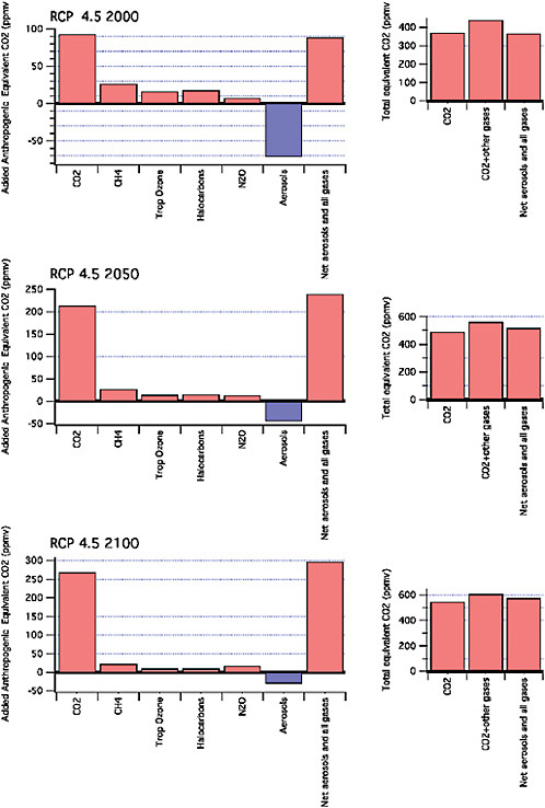
Figure 2.7 shows the CO2-equivalent concentrations for these two scenarios at three points in time. Notice that in the case of the tighter radiative forcing goal, there is some “overshoot”. That is, the target is exceeded in the middle part of the century and then gradually approached. This is due to the assumption that there will be a “negative” emitting technology, Bioenergy with Carbon Capture and Sequestration (BECS). Otherwise a faster decline rate of the capital stock would be required.
2.3
SHORT-LIVED RADIATIVE FORCING AGENTS: PEAK TRIMMING VERSUS BUYING TIME
The role of CO2 emissions in Earth’s climate future is unique among the major radiative forcing agents, because the impact of the CO2 emitted into the atmosphere will continue to alter Earth’s energy budget for millennia to come. As noted above, Earth’s energy budget is also subject to the influence of a number of short-lived radiative forcing agents whose radiative effect would decay to zero on a time scale of weeks to decades if their sources where shut off. These agents include aerosols, black carbon on snow or ice, and methane.
Aerosols are produced by burning biomass and fossil fuels, but unlike CO2 they are not an inevitable by-product of combustion. Some aerosols reflect energy to space, but other aerosols such as black carbon absorb sunlight. Reflecting aerosols unambiguously lead to cooling of the surface. Their effect has offset a portion of the radiative forcing from the anthropogenic increase of greenhouse gases so far, and any action that reduces reflecting aerosol emissions will lead to a nearly immediate warming. The effect of airborne absorbing aerosols is more subtle, because they primarily act to shift the absorption of solar radiation from the surface to the interior of the atmosphere, leaving the top-of-atmosphere energy budget largely unchanged (Randles and Ramaswamy, 2008). The global mean effect of surface black carbon is difficult to quantify but is unambiguously a warming, amplified further by the albedo feedback of melting snow and ice (Flanner et al., 2007; Hansen and Nazarenko, 2004; McConnell et al., 2007). Aerosol effects can include direct damage to human health and agriculture, implying that they should be cleaned up for reasons independent of climate (Agrawal et al., 2008; Ramanathan et al., 2008). A key question is whether the effort to do so will help or hurt other efforts to keep warming in check. Although the discussion of aerosol effects will be based primarily on temperature changes, it should be kept in mind that the spatially inhomogeneous radiative forcing from aerosols can lead to regional effects such as changes in clouds and the
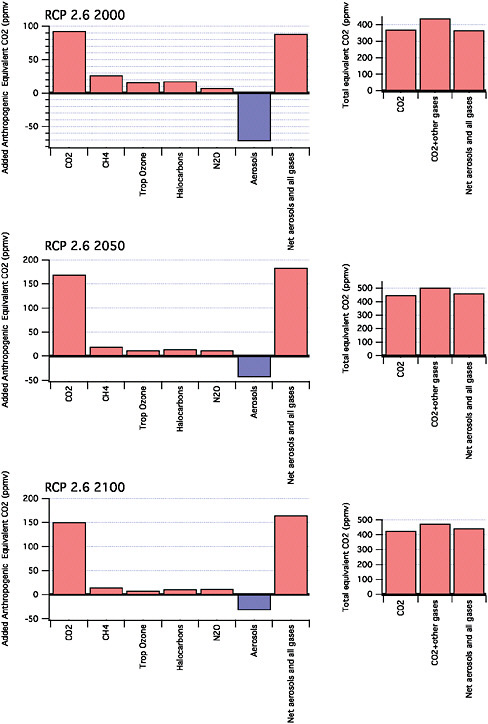
FIGURE 2.7 This figure illustrates components of radiative forcing (in CO2-equivalent concentration units) for the RCP 2.6 (a) and RCP 4.5 (b) scenarios (see Moss et al., 2010). RCP 2.6 peaks at 3 W/m–2 before 2100 and then declines. There is some “overshoot” where the target is exceeded and is then gradually approached (see footnote 1). RCP 4.5 stabilizes at 4.5 W/m–2 after 2100.
hydrological cycle. These changes constitute an anthropogenic imprint on climate that is distinct from that associated with the overall warming due to greenhouse gases.
Methane is currently emitted by a diverse set of anthropogenic sources, many of which are related to agriculture. Once in the atmosphere, methane oxidizes to CO2 with a time scale of about a decade. Since one molecule of CO2 has much less radiative effect than a molecule of methane, for methane concentrations in the present low range, the resulting CO2 is negligible in comparison to the CO2 emitted by deforestation and fossil fuel burning. In contrast to CO2, the climate effect of current anthropogenic methane emissions would decay relatively rapidly if emissions were to cease, as depicted in Figure 2.8. But it seems difficult to bring anthropogenic methane emissions to zero in the long term, given the continuing need for agriculture to feed the world’s population. A continued long-term warming contribution from methane should therefore be anticipated, not because of persistence of methane in the atmosphere, but because of likely persistence of the source. For the much more massive methane release that could come from clathrate destabilization (see Section 6.1), the CO2 produced by oxidation could have an important effect on climate.
The climate effects of short-lived radiative forcing agents are thus more reversible than those of CO2, and therefore actions reducing emissions of short-lived agents have different implications for Earth’s climate future than actions that affect CO2 emissions. Insofar as it is perceived that control of methane or black carbon may be technically easier or less economically disruptive than controlling CO2 emissions, mitigation of the short-lived warming influences has sometimes been thought of as a way of “buying time” to put CO2 emission controls into place. This is a fallacy. While one does buy a rapid reduction by reducing methane or black carbon emissions, this has little or no effect on the long-term climate, which is essentially controlled by CO2 emissions because of the persistence of CO2 in the atmosphere. The situation is illustrated schematically in Figure 2.8. The time course of warming produced by CO2 emissions alone is given schematically by the black line. If one adds short-lived radiative forcing agents with an aggregate warming effect into the mix, the effect will be to add to the temperature increase until such time as the emissions are brought under control, where after the temperature will quickly drop back to the CO2-only curve (the blue and red solid lines on the curve, representing early or delayed mitigation of short-lived forcing agents). The effect of mitigation of methane and black carbon is thus to trim the peak warming rather than limit the long-term warming to which Earth is subjected. If the early action to mitigate methane emissions
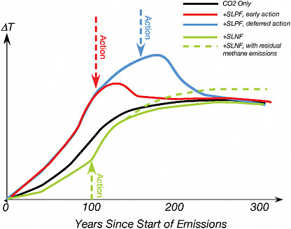
FIGURE 2.8 Qualitative sketch of the time-course of future temperature under various scenarios for control of emissions of short-lived radiative forcing agents. The time axis is given as time since the beginning of significant anthropogenic emissions of greenhouse gases. It is assumed that CO2 emissions are brought to zero after 200 years. SLPF refers to short-lived positive forcing agents, like methane or black carbon on snow or ice. SLNF refers to short-lived negative forcing agents, primarily aerosols. “Early Action” refers to a scenario in which early, aggressive action is taken to mitigate emission of short-lived radiative forcing agents, while “Deferred Action” refers to a scenario in which such actions are delayed. The green line shows what happens if the aggregate of all short-lived forcings brought under control originally added up to a cooling effect (so that reducing them warms the climate). The dashed green line is similar, except that it assumes there is a residual methane emission that cannot be reduced to zero. The cumulative CO2 emissions are assumed to be the same in all of these scenarios.
was done instead of actions that could have reduced net cumulative carbon emissions, the long-term CO2 concentration would be increased as a consequence. Peak trimming in that case would come at the expense of an increased warming that will persist for millennia. Carbon emission control and short-term forcing agent control are two separate control knobs that affect entirely distinct aspects of Earth’s climate and should not be viewed as substituting for one another.
It would be unrealistic to contemplate policies that would reduce black carbon emissions while leaving reflecting aerosol emissions intact, given that the diverse sources of emission yield an interlinked stew of absorbing and
reflecting aerosols (Ramanathan et al., 2008). The green curve in Figure 2.8 shows what happens if the aggregate of all aerosols brought under control sums to a cooling effect before mitigation; the mitigation in this case accelerates the approach to the CO2-only curve, as the masking effect of the aerosols is eliminated. If the long-term situation instead includes a recalcitrant methane emission rate that is stabilized but not brought to zero, then the long-term warming is brought above the CO2-only case for a period as long as the methane emissions continue.
2.4
CARBON CYCLE
The evolution of atmospheric carbon dioxide concentrations depends on the balance of human emissions, natural processes that remove excess carbon dioxide from the atmosphere, and the sensitivity of land and ocean carbon reservoirs to climate change and land use (see Box 2.2). The historical atmospheric growth rate of carbon dioxide is well-constrained for the past 50 years from direct instrumental measurements and for periods prior to that from measurements of gases trapped in ice cores. Global average atmospheric CO2 has risen from a pre-industrial level of about 280 ppm to about 390 ppm by the beginning of 2010. A definitive anthropogenic origin for the excess carbon dioxide can be assigned based on contemporaneous changes in carbon isotopes, a parallel decrease in atmospheric oxygen, and by the fact that the atmospheric carbon dioxide levels for the preceding several millennia of the Holocene had hovered within plus or minus 5 ppm of the pre-industrial value. Past fossil fuel combustion rates and carbon emissions from cement production and land-use change (e.g., deforestation, shifting land into pasture and agriculture) can be reconstructed, and net land and ocean carbon sources and sinks can be quantified from a combination of observations and numerical models. Figure 2.9 presents a recent synthesis for the global carbon system showing the fluxes between the atmosphere and various reservoirs versus time (Le Quéré et al., 2009). The terrestrial carbon fluxes are partitioned with carbon emissions from direct human land-use change including recovery from earlier human land use, separated from terrestrial carbon sinks in response to elevated CO2 and climate.
The response of the global carbon cycle to human perturbations can be characterized by the airborne CO2 fraction, the fraction of the cumulative carbon dioxide emitted by fossil fuel combustion and land-use change that remains in the atmosphere. The contemporary airborne fraction is currently slightly less than half (~0.45), and for any specified carbon emission trajectory, future atmospheric carbon dioxide concentrations depend on the

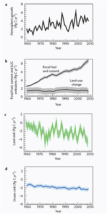
FIGURE 2.9 Components of the global CO2 budget. (a) The atmospheric CO2 growth rate. (b) CO2 emissions from fossil fuel combustion and cement production and from land-use change. (c) Land CO2 sink (negative values correspond to land uptake). (d) Ocean CO2 sink (negative values correspond to ocean uptake). The land and ocean sinks (c,d) are shown as an average of several models normalized to the observed mean land and ocean sinks for 1990-2000. The shaded area is the uncertainty associated with each component. Adapted from Le Quéré et al. (2009).
airborne fraction and how it evolves with time. At present, the ocean and the land biosphere contribute about equally to the drawdown of excess carbon dioxide from the atmosphere. Theoretical arguments and numerical models suggest that the efficiency of both the land and ocean carbon sinks may decline in the future under warmer climate conditions, which would act to amplify climate warming (Fung et al., 2005; Friedlingstein et al., 2006). The magnitude of the climate-carbon cycle feedback, however, varies substantially across model simulations and is a substantial uncertainty in future climate projections.
Excess atmospheric carbon dioxide dissolves in surface seawater as inorganic carbon through well-known physical-chemical reactions. The distribution and global inventory of anthropogenic carbon dioxide in the ocean are well characterized based on global ship-based observations collected during the late 1980s and 1990s (Sabine et al., 2004). Ongoing measurements at time-series sites and along ocean sections constrain uptake over decadal time periods (IOC, 2009). Oceanic anthropogenic CO2 uptake up to present has been governed primarily by atmospheric CO2 concentrations and the rate of ocean circulation that exchanges surface waters equilibrated with elevated CO2 levels with subsurface waters. In particular, key pathways include the ventilation of the wind-driven thermocline and deep and intermediate water formation. Ocean models constrained by field data provide estimates of the oceanic transport and air-sea flux of anthropogenic CO2 as well as reconstructions of past ocean uptake and projections for the future (Matsumoto et al., 2004; Gruber et al., 2009; Khatiwala et al., 2009).
Future ocean uptake of anthropogenic carbon is expected to decrease in efficiency (i.e., absorb a smaller fraction of the emissions); the ocean CO2 sink is expected to continue to increase, but more slowly than the emissions. Under elevated CO2, the chemical buffer capacity of seawater decreases, lowering the amount of inorganic carbon absorbed when surface waters are equilibrated with the atmosphere. Upper-ocean warming reduces the solubility of carbon dioxide in seawater. Anthropogenic CO2 uptake will be further reduced because of increased vertical stratification, reduced ocean ventilation rates, and reduced deep and intermediate water formation rates, which are expected due to warming in the tropics and subtropics and increased freshwater input in temperate and polar regions due to elevated precipitation and sea-ice melt (Sarmiento et al., 1998). In contrast, an increase in the strength of Southern Ocean winds, associated with a more positive phase of the Southern Annular Mode, may increase future uptake of anthropogenic CO2 (Russell et al., 2006).
Ocean biogeochemistry plays an important role in ocean carbon stor-
age, and biogeochemical responses to changing ocean circulation also need to be considered when assessing future net carbon uptake. The inorganic carbon concentration in subsurface ocean waters is generally elevated over surface concentrations because of the downward transport and subsequent respiration of organic water originally produced in the surface layer. In coupled carbon-climate models, biogeochemical feedbacks to a warmer climate tend to partially offset physical-chemical effects and act to reduce the overall strength of ocean climate-carbon cycle feedbacks. In the Southern Ocean, enhanced outgassing of natural CO2 due to stronger winds and upwelling may more than compensate for increased anthropogenic CO2 uptake, leading to a net reduction in ocean uptake (Le Quéré et al., 2008; Lovenduski et al., 2007, 2008). Recent observations of the air-sea difference in the partial pressure of carbon dioxide, the driving force for air-sea CO2 exchange, indicate a weakening of oceanic uptake in a number of regions, although there remains some debate whether this signal should be attributed to climate change, ozone depletion, or primarily decadal climate variability (Le Quéré et al., 2009; Watson et al., 2009).
It is more difficult to directly constrain, on a global scale, the net fluxes of carbon into and out of the more heterogeneous terrestrial carbon reservoirs, and terrestrial uptake is often estimated from a combination of terrestrial biogeochemical models and satellite remote sensing approaches that have been assessed using process experiments, local CO2 flux towers, etc. (Canadell et al., 2007; Raupach et al., 2007; Le Quéré et al., 2009). Land carbon uptake can be computed in a top-down fashion by difference from the estimated fluxes to the atmosphere, the ocean sink, and the growth rate in the atmosphere. Slightly more sophisticated approaches utilize the spatial and temporal variations in atmospheric CO2 with transport models to infer land and ocean surface fluxes (Rödenbeck et al., 2003; Peylin et al., 2005). Atmospheric carbon isotope and oxygen/nitrogen ratios also provide critical constraints on the partitioning of carbon uptake between the ocean and land biosphere (Rayner et al., 1999).
The contemporary land carbon budget is governed by a combination of interacting natural and anthropogenic processes rather than any single mechanism (Pacala et al., 2001; Schimel et al., 2001). Deforestation and biomass burning result in net CO2 fluxes to the atmosphere as high-carbon forests are turned into comparatively low-carbon pastures and croplands (Houghton, 2003). This process is now occurring mainly in the tropics and is partially countered by temperate regrowth on abandoned farm and pasture-land (Shevliakova et al., 2009). The impacts of land-use change can extend for decades after the initial disturbance, and contemporary land
carbon fluxes may reflect as much aggregate events in the past as current conditions, complicating the task of deconvolving underlying mechanisms. Experimentally, fertilization of photosynthesis by higher atmospheric carbon dioxide levels increases plant growth, in many cases substantially, and contributes to carbon uptake. When included in global models, CO2 fertilization leads to a modest current sink that may continue for many decades into the future. Some studies suggest, however, that this effect may be smaller than earlier thought perhaps due to other limitations such as nitrogen (Long et al., 2006; Thornton et al., 2009a). Many Northern Hemisphere ecosystems are also nitrogen limited, and deposition of reactive nitrogen mobilized by fossil fuel combustion may also cause increased carbon uptake (Lamarque et al., 2005; Thornton et al., 2009a). Land carbon storage varies on interannual time scales due to climate variability and in particular variations in temperature, precipitation, and water availability (Sitch et al., 2008). Wildfire also plays a major role in the global carbon cycle (Randerson et al., 2006), and increased tropical fire associated with El Niño droughts may contribute to increases in the growth rate of atmospheric carbon dioxide concentrations during recent El Niño years (Van der Werf et al., 2006).
Climate warming may cause land ecosystems to lose carbon because respiration is more temperature sensitive than photosynthesis, but there is a wide range of estimates for the climate sensitivity of land carbon stocks. Larger effects could come if future climates lead to additional disturbances, especially fire, pests, or widespread replacement of forests to grasslands, which could rapidly release large amounts of carbon. Current attention is focusing on both the role of human and climate-caused disturbance in controlling future ecosystem carbon storage and on physiological processes, such as carbon dioxide fertilization. Water availability to support photosynthesis and primary productivity is thought to be significant, with models (Fung et al., 2005) and observations (Angert et al., 2005) indicating that decreasing water balance (drier soil conditions) decreases carbon uptake. Global effects are a balance between warmer conditions favoring a longer growing season in the Northern Hemisphere temperate zone, increasing carbon uptake, and drier soils in the tropics, decreasing carbon uptake (Fung et al., 2005; Friedlingstein et al., 2006). Past and future land-use change will also affect land carbon storage and needs to be considered when projecting future atmospheric CO2 levels.
The combined effects of ocean and land feedbacks have been explored in a series of coupled climate-carbon models reported by the international C4MIP (Coupled Climate-Carbon Cycle Model Intercomparison Project; Friedlingstein et al., 2006; Figure 2.10). Simulations are conducted for the
20th and 21st centuries forced with specified trajectories for fossil fuel and land-use CO2 emissions; carbon-climate sensitivity is assessed by comparing simulations with and without coupling between model atmospheric CO2 and atmospheric radiation (and thus climate). Some simulations exhibit a large amplifying effect whereby climate effects lead to increased release of carbon dioxide, mostly from terrestrial processes. By the year 2100, simulations with strong feedbacks have higher atmospheric CO2 levels as much as 200 ppm above the companion simulation without climate feedbacks. The airborne CO2 fraction tends to increases in models where uptake processes are more sensitive to climate, where uptake processes are less sensitive to atmospheric CO2, and where physical climate sensitivity to CO2 is large.
The land modules in the C4MIP simulations did not include interactions between carbon and other limiting nutrients such as nitrogen. When soil organic matter is respired due to warming, nitrogen is released, stimulating enhanced plant growth that can offset the CO2 released from the soil matter. More recent coupled simulations that include this effect indicate a small negative climate-carbon feedback on atmospheric CO2 (Thornton et al., 2009a). Interestingly, the carbon-nitrogen model had only a very weak CO2 fertilization effect on land photosynthesis because of nitrogen limitation. As a result, the model land carbon uptake responded only weakly to rising atmospheric CO2 and had as a result one of the largest atmospheric CO2 levels at the end of the 21st century. The degree to which CO2 fertilization is modulated by nitrogen is an important unresolved science question, and for the carbon cycle, sensitivity of the sinks to CO2 is as important as sensitivity to climate. The C4MIP simulations did not address the full suite of interactions between the carbon cycle and other changes in the Earth System; for example, ocean carbon storage can be influenced by ozone-driven changes in Southern Ocean winds (Le Quéré et al., 2008; Lovenduski et al., 2008; Lenton et al., 2009). Finally, the current generation of coupled climate-carbon cycle models neglect a number of carbon reservoirs, such as high-latitude peats, permafrost and methane clathrates that could be important on longer time scales (see Section 6.1).
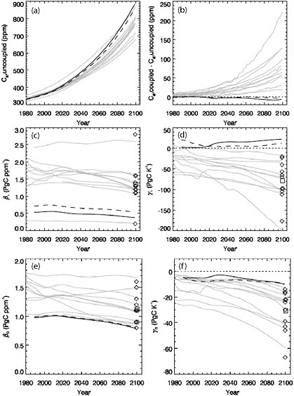
FIGURE 2.10 Predicted atmospheric CO2 and climate-carbon cycle feedback parameters. (a) Atmospheric CO2 trajectories for simulations with the same prescribed fossil fuel emissions and no CO2-radiative feedbacks. (b) Difference in atmospheric CO2 due to radiative coupling. (c) Land biosphere response to increasing atmospheric CO2. (d) Land biosphere response to increasing temperature. (e) Ocean response to increasing atmospheric CO2. (f) Ocean response to increasing temperature. Gray lines show results from carbon-only model studies from Friedlingstein et al. (2006) (also reported in IPCC, 4th assessment). Thick black lines are from a nitrogen-carbon model (Thornton et al., 2009a); thick solid line for pre-industrial nitrogen deposition and thick dashed line for anthropogenic nitrogen deposition. Diamonds show the feedback parameters estimated at year 2100 for previous studies (Friedlingstein et al., 2006), and squares show their mean. Thin dotted lines indicate zero response. (adapted from Thornton et al., 2009a).


