
5
Impacts in the Next Few Decades and Coming Centuries
5.1
FOOD PRODUCTION, PRICES, AND HUNGER
Even in the most highly mechanized agricultural systems, food production is very dependent on weather. Concern about the potential impacts of climate change on food production, and associated effects on food prices and hunger, have existed since the earliest days of climate change research. Although there is still much to learn, several important findings have emerged from more than three decades of research.
It is clear, for example, that higher CO2 levels are beneficial for many crop and forage yields, for two reasons. In species with a C3 photosynthetic pathway, including rice and wheat, higher CO2 directly stimulates photosynthetic rates, although this mechanism does not affect C4 crops like maize. Secondly, higher CO2 allows leaf pores, called stomata, to shrink, which results in reduced water stress for all crops. The net effect on yields for C3 crops has been measured as an average increase of 14% for 580 ppm relative to 370 ppm (Ainsworth et al., 2008). For C4 species such as maize and sorghum, very few experiments have been conducted but the observed effect is much smaller and often statistically insignificant (Leakey, 2009).
Rivaling the direct CO2 effects are the impacts of climate changes caused by CO2, in particular changes in air temperature and available soil moisture. Many mechanisms of temperature response have been identified, with the relative importance of different mechanisms varying by location, season, and crop. Among the most critical responses are that crops develop more quickly under warmer temperatures, leading to shorter growing periods and lower yields, and that higher temperatures drive faster evaporation of water from soils and transpiration of water from crops. Exposure to extremely high temperatures (e.g., > 35ºC) can also cause damage in photosynthetic, reproductive, and other cells, and recent evidence suggests that even short exposures to high temperatures can be crucial for final yield (Schlenker and Roberts, 2009; Wassmann et al., 2009).
A wide variety of approaches have been used in an attempt to quantify yield losses for different climate scenarios. Some models represent individual processes in detail, while others rely on statistical models that, in theory, should capture all relevant processes that have influenced historical variations in crop production. Figure 5.1 shows model estimates of the combined effect of warming and CO2 on yields for different levels of global temperature rise. It is noteworthy that although yields respond nonlinearly to temperature on a daily time scale, with extremely hot days or cold nights weighing heavily in final yields, the simulated response to seasonal warming is fairly linear at broad scales (Lobell and Field, 2007; Schlenker and Roberts, 2009). Several major crops and regions reveal consistently negative temperature sensitivities, with between 5-10% yield loss per degree warming estimated both by process-based and statistical approaches. Most of the nonlinearity in Figure 5.1 reflects the fact that CO2 benefits for yield saturate at higher CO2 levels.
For C3 crops, the negative effects of warming are often balanced by positive CO2 effects up to 2-3ºC local warming in temperate regions, after which negative warming effects dominate. Because temperate land areas will warm faster than the global average (see Section 4.2), this corresponds to roughly 1.25-2ºC in global average temperature. For C4 crops, even modest amounts of warming are detrimental in major growing regions given the small response to CO2 (see Box 5.1 for discussion of maize in the United States).
The expected impacts illustrated in Figure 5.1 are useful as a measure of the likely direction and magnitude of average yield changes, but fall short of a complete risk analysis, which would, for instance, estimate the chance of exceeding critical thresholds. The existing literature identifies several prominent sources of uncertainty, including those related to the magnitude of local warming per degree global temperature increase, the sensitivity of crop yields to temperature, the CO2 levels corresponding to each temperature level (see Section 3.2), and the magnitude of CO2 fertilization. The impacts of rainfall changes can also be important at local and regional scales, although at broad scales the modeled impacts are most often dictated by temperature and CO2 because simulated rainfall changes are relatively small (Lobell and Burke, 2008).
In addition, although the studies summarized in Figure 5.1 consider several of the main processes that determine yield response to weather, several other processes have not been adequately quantified. These include responses of weeds, insects, and pathogens; changes in water resources available for irrigation; effects of changes in surface ozone levels; effects of
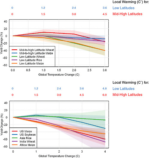
FIGURE 5.1 Average expected impact of warming + CO2 increase on crop yields, without adaptation, for broad regions summarized in IPCC AR4 (left) and for selected crops and regions with detailed studies (right). Shaded area shows likely range (67%). Impacts are averages for current growing areas within each region and may be higher or lower for individual locations within regions. Temperature and CO2 changes for the IPCC summary (left) are relative to late 20th century, while changes estimated for regions (right) were computed relative to pre-industrial. Estimates were derived from various sources (Matthews et al., 1995; Lal et al., 1998; Easterling et al., 2007; Schlenker and Roberts, 2009; Schlenker and Lobell, 2010) (see methods in Appendix for details).
|
BOX 5.1 HOW WILL MAIZE YIELDS IN THE UNITED STATES RESPOND TO CLIMATE CHANGES? Nearly 40% of global maize (or corn) production occurs in the United States, much of which is exported to other nations. The future yield of U.S. maize is therefore important for nearly all aspects of domestic and international agriculture. Higher temperatures speed development of maize, increase soil evaporation rates, and above 35ºC can compromise pollen viability, all of which reduce final yields. High temperatures and low soil moisture during the flowering stage are especially harmful as they can inhibit successful formation of kernels. In northern states, warmer years generally improve yields as they extend the frost-free growing season and bring temperature closer to optimum levels for photosynthesis. The majority of production, however, occurs in areas where yields are favored by cooler than normal years, so that warming associated with climate change would lower average national yields. The most robust studies, based on analysis of thousands of weather station and harvest statistics for rainfed maize (>80% of U.S. production), suggest a roughly 7% yield loss per ºC of local warming, which is in line with previous estimates (USCCSP, 2008b). Given the rate of local warming in the Corn Belt relative to global average, this implies an 11% yield loss per ºC of global warming (Figure 5.1). Whether these losses are realized will depend in large part on the effectiveness of adaptation strategies, which include shifts in sowing dates, switches to longer maturing varieties, and |
increased flood frequencies; and responses to extremely high temperatures. Moreover, most crop modeling studies have not considered changes in sustained droughts, which are likely to increase in many regions (Wang, 2005; Sheffield and Wood, 2008), or potential changes in year-to-year variability of yields. The net effect of these and other factors remains an elusive goal, but these are likely to push yields in a negative direction. For example, recent observations have shown that kudzu (Pueraria lobata), an invasive weed favored by high CO2 and warm winters, has expanded over the past few decades into the Midwest Corn Belt (Ziska et al., 2010).
Adaptation responses by growers are also poorly understood and could, in contrast, reduce yield losses. For example, temperate growers are likely to shift to earlier planting and longer maturing varieties as climate warms, and models suggest this response could entirely offset losses in certain situations. More commonly, however, these adaptations will at best be able to offset 2ºC of local warming (Easterling et al., 2007), and they will be less effective in tropical regions where soil moisture, rather than cold temperatures, limits the length of the growing season. Very few studies have considered the evidence for ongoing adaptations to existing climate trends and quantified the benefits of these adaptations.
|
development of new seeds that can better withstand water and heat stress and better utilize elevated CO2. A wide range of maize varieties are currently sown throughout the country, customized to local factors such as latitude, growing season length, and soil, and new varieties are continually developed by private seed companies. These companies have historically focused on biotic stresses, but are now releasing the first varieties explicitly targeted for drought resistance. Heat tolerance has not received much investment outside of drought-related traits, likely because of limited economic incentives in current climate. A comparison of maize yields in northern and southern states suggests minimal historical adaptation to heat, as varieties that are more frequently exposed to temperatures above 30ºC exhibit similar sensitivities to varieties grown in the North (Schlenker and Roberts, 2009). A major challenge in developing drought and heat tolerance is that traits that confer these often reduce yields in good years, and growers and seed companies have little economic incentive to accept this trade-off given current markets and insurance programs. Another persistent challenge is the decade or more lag between initial investments and seed release. In short, adaptation could offer large benefits, but only if formidable technical and institutional barriers are overcome. To put the challenge in context, global cereal demand is expected to rise by roughly 1.2% per year (FAO, 2006), so that adapting to 1ºC global warming (or avoiding 11% yield loss) is equivalent to keeping pace with roughly 9 years of demand growth. The corresponding expected impact of 2ºC global warming is 25%, or roughly 20 years of demand growth. |
Future development of new varieties that perform well in hot and dry conditions may also promote adaptation, but again the extent to which this will help remains unclear. Breeders and geneticists must continually weigh trade-offs between producing ample yield under stressful conditions and producing high yields under favorable conditions (Campos et al., 2004). At the higher warming levels considered in this report, it will be increasingly difficult to generate varieties with a physiology that can withstand extreme heat and drought while still being economically productive.
Although most studies have focused on crops, effects of climate change on livestock, aquaculture, and fisheries have also been considered in recent years. Livestock in parts of the world are raised mainly on grain and oilseed crops, in which case impacts will largely follow from the prices of these commodities and the costs of cooling or losing animals during heat waves. In other cases livestock depend on grazing pasture and rangeland grasses, which follow a similar pattern to crops in that temperate regions will see modest gains up to ~2ºC local warming, although forage quality may decrease with higher CO2 (Easterling et al., 2007). Although livestock systems are vulnerable in tropical areas, they may become increasingly relied upon as a strategy to cope with greater risks of crop failures (Thornton et al.,
2009b). As with livestock, impacts on fisheries are still very uncertain, but a recent study suggests that if global average warming were to be 2ºC, catch potential could rise by 30-70% in high latitudes and fall by up to 40% in the tropics, as commercial species shift away from the tropics as the ocean warms (Cheung et al., 2010).
Food Prices and Food Security
One of the strengths of a global food system is that shortfalls in one area can be offset by surpluses in another. Models of the global food economy suggest that trade will represent an important but not complete buffer against climate change-induced yield effects (Easterling et al., 2007). Specifically, the comparative advantage will shift toward regions currently below optimum temperatures for cereal production (e.g., Canada) and away from hot tropical nations, with greater flows of food trade from north to south. On average, studies suggest small price changes for cereals up to 2.5ºC global temperature increase above pre-industrial levels, with significant increases for further warming, but there is considerable uncertainty around these estimates (see Box 5.2).
Implications of climate change for hunger, or the more technical term—food insecurity—follow in part from price changes, but also depend critically on how sources of income and other aspects of health are affected by climate. A useful rule of thumb provided by early studies suggested that malnourishment would rise by roughly 1% for each 2-2.5% rise in cereal prices (Rosenzweig, 1993). These and subsequent analyses often make untested assumptions about the ability of poor tropical nations to maintain economic growth in the face of declining agricultural productivity. For example, many African countries rely on agriculture for half or more of all economic activity, and losses in productivity could dampen purchasing power. Conversely, where price rises are greater than yield losses, households dependent on agricultural income could see net gains in food security. In general, rural and urban workers with little or no landholdings are the most vulnerable to price shocks. A new generation of models that explicitly account for income sources among poor populations is emerging but yet to provide robust insights. Also important could be climate-induced changes in the incidence of diarrheal and other diseases, which inhibit food security by reducing utilization of nutrients in food.
|
BOX 5.2 CLIMATE CHANGE IMPACTS ON GLOBAL CEREAL PRICES Several modeling groups have analyzed future changes in global cereal markets in response to climate change. All operate by making estimates of yield responses in each region, and then inputting these into a model of global trade that computes the optimal mix of crop areas in different regions and the market-clearing price. Five models summarized by the recent IPCC report suggests small price changes for warming up to 2.5ºC, and a nonlinear increase in prices thereafter (Easterling et al., 2007). Two important caveats relate to these estimates, however. First, the yield changes used in these models usually assume considerable levels of farm-level adaptations, which substantially reduce impacts. For example, in one prominent study cereal prices rose by 150% for a 5.2ºC global mean temperature rise if farm-level adaptations were not included. When changes in planting dates, cultivar choices, irrigation practices, and fertilizer rates were simulated, these price changes were reduced to roughly 40% (Rosenzweig and Parry, 1994). Other studies often do not estimate impacts without adaptation, making it difficult to gauge assumptions. The costs of adaptation are also not considered in these studies, or reflected in price changes. Second, most assessments have not adequately quantified sources of uncertainty. Although different climate scenarios are often tested, processes related to crop yield changes and economic adjustments are often implicitly assumed to be perfectly known. An additional source of uncertainty is potential competition with bio-energy crops for suitable land, which could limit the ability of croplands to expand in temperate regions as simulated by most trade models.m |
5.2
COASTAL EROSION AND FLOODING
Our knowledge of the links between atmospheric concentration limits, trajectories toward equilibrium temperature change, and sea level rise is fraught with uncertainty. As reported in Section 4.8, it is therefore only possible to offer a range of sea level rise between 0.5 and 1.0 m through 2100.
Moving down the causal chain to consider coastal erosion and flooding adds yet another layer of complication because both are driven primarily by storm surges, land-use decisions, and other processes whose intensities and frequencies change from place to place. These changes alter the characters of associated risks even if changes in the intensities and frequencies of the storms, themselves, cannot be projected. The social and economic ramifications of these physical manifestations of climate change depend critically on patterns of future development and population growth. It is, therefore, extremely difficult to offer credible broad-based estimates of vulnerabilities and potential adaptation costs. At best, in fact, we can offer only suggestive
ranges of aggregate risk and more quantitative estimates only for specific locations.
Figure 5.2 offers a portrait of the geographic spread of deltas and mega-deltas where mega-cities are at the greatest risk from rising seas—these are the “hot-spots” of “key vulnerabilities” in the coastal zone. Ericson et al. (2006) estimated that nearly 300 million people currently inhabit a sample of 40 such deltas with an average population density of 500 people per km2.
Translating this observation into projections of future vulnerabilities, Table 5.1 shows the sensitivity of estimates of populations subject to coastal flooding in 2080 to assumptions about socioeconomic development as described in the SRES scenarios—sensitivity generated by differences across the scenarios in population growth and by differences in assumptions about economic development and therefore the capacity to adapt. Figure 5.3 emphasizes the importance of adaptation when it suggests, for example that 1 m of sea level rise could put between 10 and 300 million more people at risk of coastal flooding each year. It is important to note, in interpreting this figure, that the likelihood of inundation from coastal storms may not be proportional with sea level rise. Moreover, the consequences of these storm events calibrated in millions of people in jeopardy from coastal flooding depend on local population densities and geographic features. The result of the
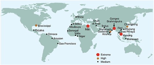
FIGURE 5.2 Relative vulnerability of coastal deltas as shown by the indicative population displaced by current sea-level trends to 2050 (Extreme=>1 million; High=1 million to 50,000; Medium=50,000 to 5,000; following Ericson et al., 2006). Source: Nicholls et al. (2007: Figure 6.6).
TABLE 5.1 Regional Distribution of Population Subject to Coastal Flooding in 2080 along Alternative SRES Scenarios.
|
|
|
NOTE: Population estimates by region assume proportional population growth within coastal regions. Source: Nicholls (2004) as displayed in Nicholls et al. (2007: Table 6.5). |
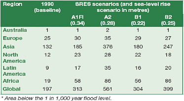
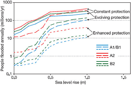
FIGURE 5.3 Estimates of people flooded in coastal areas attributable to sea level rise along alternative SRES scenarios. Estimates of the number of additional people in jeopardy from coastal flooding along alternative SRES development scenarios for three gross categories of adaptation intensities are displayed. Constant protection envisions maintaining current practices, evolving protection envisions increasing protection as local economies grow to preserve the current pattern with respect to national GDP, and enhanced protection envisions accelerating the pace of adaptation so that increasing resources are devoted to protection. Source: Nicholls et al. (2007: Figure 6.8) derived from Nicholls and Tol (2006).
confluence of these complications is a noticeable threshold of accelerating risk around 0.3 m of sea level rise that is captured even by global aggregates regardless of adaptation effort. As a result, even 50 cm of SLR could put between 5 and 200 million more people annually at risk of flooding.
Tol (2007) used a specific integrated assessment model of his own creation to portray aggregate measures of erosion that parallel estimates of populations facing complete displacement and/or significant economic loss derived from economically efficient abandonment and/or growing protection costs across developed and developing countries. Figure 5.4 calibrates his results graphically in relation to sea level rise; they were derived from a socioeconomic portrait that was crafted to be consistent with the IS92a emissions scenario for which seas rise by roughly 60 cm through 2100. This work suggests that 50 cm of sea level rise could permanently displace up to 4 million people and cause more than 250,000 km2 of wetland and dry-land to be lost to erosion worldwide (with 90% of these losses projected to occur in developing countries). The human faces behind the global displacement results portrayed here can, of course, be seen in examples of erosion from coastal storms and rising seas. In the Arctic, Newtok, Alaska is already preparing for complete displacement, for example, and several neighboring towns face the same fate in the near future. Meanwhile, many small island states like Tuvalo, the Maldives, and the Cook Islands foresee similar futures this century if sea level rise continues.
Geographic detail for physical processes like erosion and inundation
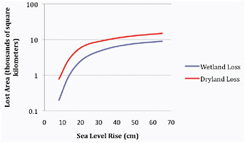
FIGURE 5.4 Losses attributable to sea level rise. Estimates of wetland and dry-land losses for developed (Panel A) and developing countries (Panel B) correlated with sea level rise along a socioeconomic scenario that tracks IS92a. Source: Derived directly from Tol (2007) as depicted in Nicholls et al. (2007: Figure 6.10).
TABLE 5.2 Selected Losses from Sea Level Rise and Associated Erosions across Asia
|
SLR Rise (from 2000 levels) |
Location |
Magnitude |
Source |
|
0.3 m |
China |
81.4 · 103 km2 |
Du and Zhang (2000) |
|
|
Huanghe-Huaihe Delta |
21.3 · 103 km2 |
|
|
|
Changjiang Delta |
54.5 · 103 km2 |
|
|
|
Zhujiang Delta |
5.5 103 km2 |
|
|
1.0 m |
Japan |
2.3 · 103 km2 |
Mimura and Yokoki (2004) |
|
1.0 m |
Korea |
1.2% area |
Madsen and Jakobsen (2004) |
|
1.1 m |
India and Bangladesh |
478 km2 (11%) |
Loucks et al. (2010) |
|
1.2 m |
India and Bangladesh |
1,396 km2 (33%) |
|
|
0.3 m |
India and Bangladesh |
4,015 km2 (96%) |
|
from sea level rise has been emerging over the past decade. Table 5.2, for example, offers estimates for several locations in Asia. Some are located in important deltas in China where modest sea level rise of 0.3 meters would cause significant loss of land area from inundation and erosion; others are located in eastern and southeastern Asia where 1 m of sea level rise would cause significant loss of land and protective mangroves in addition to putting many people at risk of displacement. The final entry reports recent estimates of associated loss in the habitat of the only tiger population in the world (panthera tigris) that is adapted to living in mangroves; Loucks et al. (2010) report that a nonlinear decline to extinction (at 30 cm) would begin around 15 cm of sea level rise.
Turning to specific locations within the United States, where it is possible to focus attention on downstream impacts and the potential adaptation, Figure 5.5 first depicts coastal vulnerability to erosion across the mid-Atlantic region at the end of the century for three sea level rise scenarios. Enormous variability from site to site along the coastline is clearly displayed; and so it is obvious that potential risks and the potential for adaptation can be expected to be equally diverse.
5.3
STREAMFLOW
Runoff is defined as the difference between precipitation and the sum of evapotranspiration and storage change on or below the land surface. On long term balance, it must be balanced by precipitation minus evapotranspiration, which also equals atmospheric moisture convergence. Streamflow is
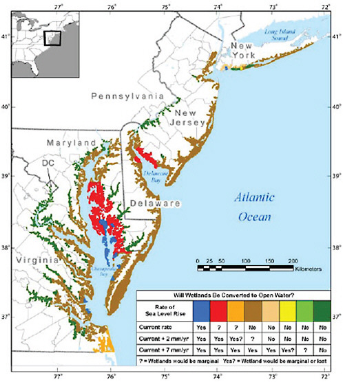
FIGURE 5.5 Wetland loss from erosion attributable to sea level rise along three alternative scenarios. Confirmation of the hypothesis that wetland and marshes would be covered to open water by the end of the century along feasible sea level rise scenarios (current trend up to almost 70cm by 2100. Source: USCCSP (2009: Figure ES.2).
runoff that moves through the channel system to a given point (in practice, often a stream gauge at which streamflow measurements are made).
Runoff is a key index of the availability of freshwater, a quantity that is essential for human life. Although on average only about 5 liters per day of water are necessary for adult survival, water use in industrialized countries is much higher—around 200 liters/day in the United States and 150 liters in Europe. On the other hand, the average for Africa is only about 10 liters, or double the minimum for survival. Total water consumption for agriculture globally is about 10 times that for municipal use (Shiklomanov, 1999). Groundwater, an important source of water in many parts of the world, makes up an additional estimated 25 percent of total global water withdrawals (International Water Management Institute, 2007). Groundwater recharge, although difficult to estimate except on a local basis, is roughly related to the excess of precipitation over evapotranspiration, and so very approximately can be taken as a fraction of annual runoff. Hence, understanding how runoff will change in a future climate is the key to understanding how water availability for human use might change.
In climate models, runoff is represented by land surface models, which have the primary purpose of partitioning net radiation at the land surface into latent, sensible, and ground heat flux. A secondary purpose (which is linked to modeling of the surface energy balance, because evapotranspiration, or equivalently latent heat, is common to the energy and water balances) is to partition precipitation into infiltration and runoff. Runoff is also produced in most models by parameterizations of subsurface hydrologic processes, albeit crudely in most models. Although many models do not consider the transformation of runoff to streamflow, a few do. On long-term (average annual) balance, runoff is roughly equal to streamflow, ignoring channel processes (such as groundwater interactions), which in most cases have modest effect.
Past attempts to understand the sensitivity of runoff and streamflow to a changing climate have followed two general pathways. The most common is to use river basin hydrological models, which typically are forced with precipitation and other surface atmospheric variables, and to prescribe differences in the forcings that reflect the effects of climate change. This approach, sometimes termed downscaling, has been applied in one of three ways. The first is the so-called delta method, which adjusts precipitation and temperature by factors or shifts that reflect climate model-estimated differences between current and future climate. An example of this approach is the study by Hamlet and Lettenmaier (1999) of the effects of climate change on the water resources of the Columbia River Basin. The second approach
is statistical downscaling, which “trains” a relationship between current climate (precipitation, surface air temperature, and other variables) produced by a climate model and observations, in such a way as to correct for climate model biases and spatial and temporal scale mismatches. The same relationship is then applied to future climate simulations. For both current and future climate, the downscaled climate model output is used to force a river basin hydrology model. Examples of this approach are the study by Hayhoe et al. (2007) of climate change impacts on the northeastern United States, the Maurer et al. (2007) study of California water resources, and Christensen and Lettenmaier’s (2007) study of Colorado River water resources. The third approach is dynamical downscaling, in which a regional climate model (RCM) is nested within a global model to produce more spatially resolved climate model output. Although dynamical downscaling may be preferred on theoretical grounds (because it is based on physical rather than statistical relationships; its application in practice has been problematic because the computational burden is high, hence the number of RCM runs that can be performed for different global models is small. Furthermore, practical constraints, like the fact that global model output sufficient to provide requisite variables at the RCM domain boundary often are not archived, or are not archived at sufficient vertical levels in the atmosphere and time resolution to meet RCM needs. Finally, Wood et al. (2004) showed that even after dynamical downscaling, application of statistical post-processing, similar to that used in statistical downscaling methods, was necessary to remove RCM bias prior to using RCM output to force a hydrological model.
The second pathway is direct analysis of global climate model runoff predictions. This approach usually has not been favored for river basin studies, because of the scale mismatch between the spatial resolution of the global models (typically several degrees latitude by longitude) and the river basin scale. However, for analysis of large river basins, Milly et al. (2005) (and replots of the Milly et al. [2005] results at the scale of the U.S. hydrologic regions in the USCCSP Synthesis and Assessment Product 4.3 [USCCSP, 2008b]) have found this approach to be useful, especially because it avoids the issues associated with downscaling and inconsistencies in fluxes at the river basin scale. Seager et al. (2007), in an analysis of projected changes in runoff over the U.S. Southwest, also analyzed GCM runoff directly.
Despite the fact that direct analysis of GCM runoff has not been widely performed, we use this approach here for two reasons. First, post processing of global model output by statistical downscaling and hydrological modeling results in a mismatch in the surface water balance between the hydrologic model that produces streamflow simulations and the global model. Second,
although some (but not all) of these issues are resolvable via dynamical downscaling, the logistical requirements for so doing make dynamical downscaling infeasible for analysis of the broad suite of GCM output in the IPCC AR4 (and upcoming AR5) archives.
We have used as our motivation here the Milly et al. (2005) study, which analyzed multidecadal runoff from 12 GCMs for mid-21st century as compared with early 20th century runoff (24 separate model runs were analyzed; however, some models had multiple ensembles, which were averaged). An important difference, however, is that for reasons articulated in Chapter 2 we performed our analysis in a way that links projected runoff changes with changes in the global mean temperature. Accordingly, we proceeded as follows. We extracted IPCC AR4 archived runoff output along with surface air temperature, precipitation, and evapotranspiration for 23 models for which global monthly output for (in most cases) 1870 through 2100 was archived. For each model and emissions scenario, we computed the global mean temperature for each year. We then computed a 30-year moving average of the global mean temperatures, and from this time series, we determined the year at which the global mean temperature was larger than for 1985 (1971-2000 mean) by 0.5ºC, 1ºC, 1.5ºC, and 2.5ºC. We then computed 30-year moving averages of runoff for each model, emissions scenario (A2, A1B, and B1), and grid cell, and overlaid the runoff values for 1985 and the year in which the moving average global temperature rise was the given amount (0.5, … 2.5) to the U.S. hydrological regions. We then computed runoff changes as percentages per degree C of global warming, and took the median over models and global temperature changes of 1ºC, 1.5ºC, and 2ºC. We also computed equivalent standard errors of the medians (see Table 5.3). Figure O.2 shows the results. In general, runoff decreases over most of the country, with the exception of the northeast and the northwest. Closer examination of similar results (not shown) for precipitation and evapotranspiration indicate that (a) changes in runoff result from a combination of slight increases in precipitation (in the multi-model median) over most of the country with the exception of the Southwest, and increasing evapotranspiration over all but the Southwest (where lower precipitation apparently limits moisture available for evapotranspiration); (b) the general patterns of changes (runoff sensitivities per degree C) are roughly constant over the range 1-2ºC global temperature rise; and (c) the patterns of changes and sensitivites per degree C are similar for the different emissions scenarios (hence justifying pooling of the results over emissions scenarios).
We also conducted a similar analysis for global runoff changes, which are also shown in Figure O.2. The figure shows (a) increases (in the multi-
TABLE 5.3 Median Runoff Sensitivities Relative to the Period 1971-2000 per Degree Global Average Temperature Change, the Equivalent Standard Error of the Median, and Fraction of Positive Minus Negative Estimates (FPN) for the U.S. Hydrologic Regions and Alaska
|
Hydrologic Region |
Median (%) |
Equivalent Std Errora (%) |
FPNb |
|
1 New_England |
1.7 |
0.6 |
0.47 |
|
2 Mid-Atlantic |
1.0 |
0.7 |
0.29 |
|
3 South_Atlantic-Gulf |
−2.0 |
1.1 |
−0.18 |
|
4 Great_Lakes |
1.7 |
1.3 |
0.15 |
|
5 Ohio |
1.5 |
1.0 |
0.24 |
|
6 Tennessee |
−2.8 |
1.1 |
−0.24 |
|
7 Upper_Mississippi |
1.2 |
1.2 |
0.09 |
|
8 Lower_Mississippi |
−6.4 |
1.7 |
−0.53 |
|
9 Souris-Red-Rainy |
1.8 |
1.6 |
0.21 |
|
10 Missouri |
−2.0 |
1.1 |
−0.12 |
|
11 Arkansas-White-Red |
−8.4 |
1.4 |
−0.56 |
|
12 Texas-Gulf |
−7.4 |
2.1 |
−0.56 |
|
13 Rio_Grande |
−12.2 |
2.3 |
−0.47 |
|
14 Upper_Colorado |
−6.3 |
1.7 |
−0.62 |
|
15 Lower_Colorado |
−6.1 |
2.4 |
−0.44 |
|
16 Great_Basin |
−5.1 |
1.4 |
−0.44 |
|
17 Pacific_Northwest |
1.2 |
0.9 |
0.24 |
|
18 California |
−3.3 |
2.2 |
−0.29 |
|
19 Alaska |
9.3 |
0.9 |
0.91 |
|
Coloradoc |
−6.2 |
1.6 |
−0.59 |
|
NOTE: The runoff sensitivity is taken as the average sensitivity (as described below) for IPCC AR4 GCM output from A2, A1B, and B1 simulations for each basin as derived from 30-year runoff averages centered on the years for which the global average (for each of 23 models and the 3 emissions scenarios) were 1ºC, 1.5ºC, and 2ºC minus the 30-year model average runoff for 1971-2000, divided by the global temperature change. The total number of model and temperature change pairs was 68, consisting of 23 models for 1ºC temperature change, 23 models for 1.5ºC temperature change, and 22 models for 2ºC temperature change. The equivalent standard error is an estimate of the standard error of the median (Hojo,1931), where “equivalent” pertains to the fact that the estimate is strictly correct only for normally distributed variates. a1.25σ/, bFraction of pairs (of 68 total) with inferred positive runoff sensitivities minus fraction with inferred negative sensitivities. FPN therefore ranges from –1 when 68 inferred sensitivites are negative, to 1 when all are positive. cUpper and Lower Colorado combined. |
|||
model median runoff sensitivity) across almost all of Eurasia, high-latitude areas, and most of Australia; (b) decreases across much of the United States, southern Europe, and Africa; and (c) (not shown) strong agreement as to the direction of runoff changes at high latitudes and southern Europe, little agreement across most equatorial areas, and only modest agreement over much of the United States (for the United States, see also the fraction positive minus fraction negative in Table 5.3).
Finally, there are some apparent differences in the pattern of runoff
changes shown for the United States in Figure O.2 relative to the re-plots of Milly et al. (2005) results in USCCSP (2008b). In general, those results showed more of an east-west divide in runoff changes across the United States, with modest increases in the east, and decreases across most of the west, which were most severe in the Colorado River and Great Basins. We extracted from our multi-model suite the same 12 models analyzed by Milly et al. (from the approximately 20 that were available to us), and analyzed the results in the same way as did Milly et al. (2041-2060 minus 1900-1970 means). When so analyzed, the results were quite similar to those shown in USCCSP (2008a). The differences in patterns in our results as compared with USCCSP (2008b) and Milly et al. (2005) apparently come about because of (a) differences in the 1900-1970 based period (used by Milly et al. [2005] versus 1971-2000 base period that we used, and (b) differences in the number of models considered (nearly double in our analysis relative to those available to Milly et al. (2005). As in Milly et al. (2005) and USCCSP (2008a), we have limited our analysis to annual runoff volumes.
Our overall conclusion therefore is that streamflow in many temperate river basins outside Eurasia will decrease as global temperature increases, with the greatest decreases in areas that are currently arid or semi-arid. Streamflow across most of the United States will decrease, although there is considerable disagreement among models aside from the Southwest, where most models project decreases, and Alaska, where most models project increases. Runoff sensitivities are approximately constant (per degree of global warming) in the range 1-2ºC warming. There is strong agreement among models that runoff in the Arctic and other high-latitude areas, including Alaska, will increase.
5.4
FIRE
The impact of climate change on the frequency of large fires and extent of area burned by wildfires depends mainly on the type of vegetation (fuel) and the future weather and climate. In many regions that have been examined, the projected climate change will cause large changes in wildfire frequency and extent. In a broad sense, wildfires will increase in regions that are dominated by forests that are already prone to fire in the current climate, while warming (without a sufficient increase in precipitation) will cause a decrease in wildfires in some shrub and grassland (fuel limited) regions that are prone to fire in the present climate.
The probability of wildfire depends on the availability of fuel, the moisture content of the fuels, and the likelihood of ignition. Ignition of most large
wildfires is by lightning, and analyses of the global lightning strike and fire frequency data suggests that ignition is a limiting variable for wildfires in only a few areas on the planet (Krawchuck et al., 2009). Once fire is initiated, the extent of a fire burn depends on fuel distribution and moisture content, wind, and topography.1 Hence, vegetation type, weather, and the antecedent weather history (climate) are the main environmental parameters that determine the frequency and extent of wildfire.
Comprehensive spatial and temporal records of wildfire and of climate variables are available for the western United States. Analyses of these data have led to a conceptual model that links wildfires to climate variability and vegetation type. For example, Westerling and Bryant (2008) found that in California and surrounding states, wildfires in “wet regions” (defined as when climatological soil moisture exceeded 28% of capacity) tended to be reported as forest fires, while wildfires in dry regions tended to be reported as grassland and shrub fires. They further found that “wet” regions were much more prone to fire in months when the maximum temperature exceeded 23ºC. Hence, they called these wet regions “energy limited”—positing the probably of fire increases with increasing temperature because the moisture content of the fuel also decreases with increasing temperature. They noted that wildfires in dry regions were positively correlated with the previous year’s precipitation—a result previously known from the study of Swetnam and Betancourt (1998)—and posited that increased moisture in the previous year allowed for an increase in biomass production in grassland environments that was then available to burn in the following summer. Hence, they called these dry regions “moisture limited”—although in the sense of moisture limiting the mass of fuel available to burn, rather than the incidence of fire. Mid-elevation regions in the Sierra were classified as “energy limited,” while southern California was classified as “moisture limited.”
Littell et al. (2009) develop empirical models for wildfire area burned throughout the western United States. For predictors, they use seasonal and antecedent climate variables including temperature and precipitation, and the Palmer Drought Severity Index (PDSI) as a proxy for soil moisture. Littell et al. formulate empirical models for zones of similar vegetation and
geography (ecoprovinces) that encompass most of the western United States2 They develop empirical models using the interannual records for the time period 1977-2003. The empirical models account for, on average, two-thirds of the variance of the wildfire area burned in the 16 ecoprovinces that comprise the western United States (cross-validated). Littell et al. find that in most of the forested western United States, wildfire area burned is best explained by dry and warm conditions in the seasons immediately preceding the fire, presumably because such climate conditions enhance evapotransporation and reduce fuel moisture. In contrast, fire area burned in the southwest United States and in other arid ecoprovinces is strongly dependent on the increased precipitation or positive PDSI (moisture) in seasons preceding the fire season, consistent with the long-standing hypothesis that extra biomass is produced in the seasons prior to the season that experiences an unusually large area burned in these regions.
Together, the studies by Littell et al. (2009), Westerling and Bryant (2008), and others demonstrate that the role of climate variability in regulating area burned is mainly a complex function of the climate (temperature, precipitation, and wind), vegetation type, and orography. Nonetheless, the climate and fire data for the United States are sufficient in spatial and temporal coverage to formulate sensible and remarkably skillful predictive models or incidence of wildfire and wildfire area burned. An example is provided in Figure 5.6 from Littell et al. (2009: Figure 1), which shows the observed wildfire area burned for the entire historical record (1916-2003) and that predicted by empirical models that are trained and cross-validated using the data from 1977-2003.
The results from the aforementioned studies strongly suggest that empirical models of wildfire should provide a skillful projection of how climate change due to increasing greenhouse gases will impact wildfire across wide regions of the globe, including the western United States and Canada. In these regions, much of the area burned is due to large wildfires that result mainly from climate variability, with in-season summer temperature, precipitation, and soil moisture being the predominant controls on fire. The probability of summer averaged temperature and humidity is relatively straightforward to quantify (precipitation perhaps a bit less so), and empirical and hydrologic models needed to project summer soil moisture are quite mature.
To date, only a few studies have examined how the projected climate
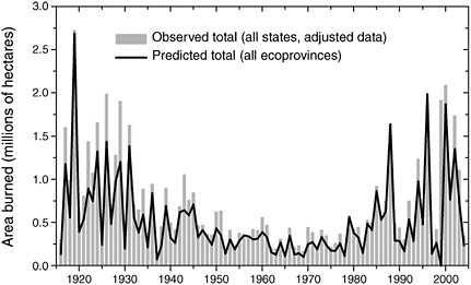
FIGURE 5.6 Observed and reconstructed wildfire area-burned for 11 western U.S. states (bars) and reconstructed (line) for the period 1916-2004. Source: Littell et al., 2009: Figure 1)
changes will impact wildfires. Shown in Figure 5.7 are the projected changes in the probability of large (> 200 ha) wildfires in 2070-2090 compared to the reference period 1961-1990 from one such study (Westerling and Bryant, 2008) that used the output from two of the AR4 climate models (GFDL and PCM) that were forced with two of the emission scenarios (B1 and A2). There are two important lessons to be learned from this plot. First, two different climate models give two very different answers for California: the PCM projects a subtle change in large wildfires everywhere, while the GFDL model projects large increases in the probability of large wildfires throughout northern California. These differences are mainly due to differences in the projected mean climate: the GFDL model features large temperature increases and precipitation decreases throughout California, while the PCM has modest temperature increases and subtle changes in precipitation. Hence, the full suite of AR4 climate models must be employed to project the probability of wildfire changes—throughout the globe. Second, although both models show increasing temperature and decreasing precipitation throughout the state of California, the likelihood of a large fire increases in northern California (especially in the Sierra) and decreases in southern California in both
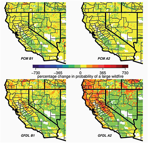
FIGURE 5.7 The projected changes in the probability of large (> 200 ha) wildfires in 2070-2090 compared to the reference period 1961-1990 using the output from two of the AR4 climate models (GFDL and PCM) that were forced with two of the emission scenarios (B1 and A2). Source: Westerling and Bryant (2008: Figure 7).
models. This reflects the fundamental differences in the climate impacts on fire regime in these regions due to differences in vegetation type.
The change in the probability of the wildfire area burned in the western United States due to increased greenhouse gases can be estimated using the methods outlined in Littell et al. (2009), modified to use temperature and precipitation as the predictor variables. Shown in Figure 5.8 is the change
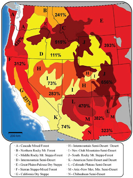
FIGURE 5.8 Map of changes in area burned for a 1ºC increase in global average temperature, shown as the percentage change relative to the median annual area burned during 1950-2003. Results are aggregated to ecoprovinces (Bailey, 1995) of the West. Changes in temperature and precipitation were aggregated to the ecoprovince level. Climate-fire models were derived from NCDC climate division records and observed area burned data following methods described in Littell et al. (2009). Sourcce: Figure from Rob Norheim.
in median annual averaged area burned in the western United States due to a 1ºC global average temperature increase, using the temperature and precipitation patterns from the corresponding figures in Chapter 4. The increase in median annual area burned ranges from 73% to over 600%, depending on the ecoprovince. Aggregating all 14 ecoprovinces in which fire is most sensitive to temperature variations, the net area burned by the median fire increases from 572,000 ha for the reference period 1970-2003, to 1,800,000 ha with a 1ºC global average temperature increase.
Other investigators using different climate models and a variety also find thata climate change will increase the risk of wildfire throughout the western United States, so long as fuel is not limiting. For example, Spracklen et al. (2009) used output from the GISS AGCM coupled to a slab ocean forced by the A1B emission scenario with an empirical model very similar to that used by Littell et al. (2009); they concluded that climate changes projected for the mid-21st century would result in a 54% increase in total annual area burned compare to that in the late 20th century, and burn areas doubling in the Rockies and Pacific Northwest.
Similar studies have been done to examine how climate change will affect forest wildfires in other regions of the world, including Australia, New Zealand, the southern Mediterranean, and in boreal forests of Canada (IPCC, 2007d). In general, these studies report wildfires will increase over the course of the century due to projected climate changes from one or more of the AR4 climate models using one or more of the marker emission scenarios.
As the time horizon increases, a further complication arises in projecting wildfires because of the importance of fuel availability and quality (moisture content) for determining the likelihood and size of wildfires. Systematic climate changes will inevitably alter the distribution of the vegetation, and significant changes in the vegetation would greatly affect the potential for wildfires and the wildfire area burned. For example, if climate change further dries already arid grasslands, then the grasslands will wither to deserts and fire will no longer be supported. On the other hand, if climate change changes the distribution of pest and pathogens such that forests become diseased, then additional fuel will be made available due to forest dieback (see, e.g., discussion of the bugs in the BC/AK spruce) and fires will be enhanced until the extra fuel is exhausted and replaced by woodlands or grasslands. To date, all of the statistical models for wildfire do not admit changes in vegetation type due to the ecosystem response to climate change.
5.5
INFRASTRUCTURE
Infrastructure and Society
Infrastructure provides a broad range of human, environmental, and economic services including buildings, transportation, waste removal and treatment, water lines, communications, and electric power grids designed to improve and sustain our society and our quality of life (Kirshen et al., 2008b). The importance of infrastructure to an industrialized economy is reflected in the magnitude of its investments: in 2007, for example, the U.S. Bureau of Economic Analysis valued the stock of all public non-defense fixed assets in the United States at approximately $8.2 trillion (Heintz et al., 2009).
Changing risk of heat waves and droughts, storms and floods, and rising sea levels are just a few of the hazards climate change poses to infrastructure (Kraas, 2008). These extreme events confront human systems and constructs with weather conditions far outside their accustomed range (Wilbanks et al., 2007). The exposure of society and infrastructure to climate change is exacerbated by the fact that much of the world’s population growth over the next few decades is likely to occur in urban areas, as they double in size from 3 to more than 6 billion from 2007 to 2050 (UN, 2008). At the same time, however, this sector has a greater ability to adapt to changing conditions than many others, as humans created the systems being affected by climate change.
In the past, other human stressors on infrastructure—from rapidly expanding urban populations to deteriorating and aging systems, many of them operating on time scales of years rather than decades—meant that climate change was rarely considered as a key influence on infrastructure costs. However, climate changes in recent decades have increased awareness regarding the risk of significant and costly impacts to infrastructure: whether from melting permafrost in the Arctic affecting roads, pipelines, and buildings, or from storm surges in the Gulf potentially flooding and damaging homes, cities, highways, and rail lines (USGCRP, 2009; Figure 5.9).
Infrastructure response to climate change is not always continuous but can be step-wise as system failure may occur above a certain threshold: whether an underpass tends to flood when more than 2.5 inches of rain falls in a 24-hour period, for example, or train rails warp only when temperatures rise above a given threshold. Local conditions can further magnify the susceptibility of cities to climate-related impacts (Wilbanks et al., 2007). High-latitude and coastal areas are uniquely vulnerable to climate change.
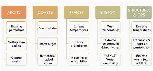
FIGURE 5.9 Climate drivers of impacts on vulnerable regions (Arctic, coasts) and sectors (transportation, energy, and buildings).
In the Arctic, protective shore ice is forming later in the year and breaking up earlier, allowing autumn storms to batter the unprotected coasts, eroding the coastline and endangering its inhabitants (ACIA, 2005). Travel over frozen ground has been cut from 7 to 4 months per year, isolating many communities (USGCRP, 2009). Under an approximate global average temperature change of 2ºC, melting of the continuous permafrost area in the Arctic characterizes infrastructure across nearly half of the Arctic land area as “high risk” and significant proportions of Arctic coastline as susceptible to significant erosion (ACIA, 2005).
At the same time, however, decreasing sea ice in the Arctic could open the Northern Sea Route, greatly reducing the distance required to transport goods between Asia, North America, and Europe. Under the same 2ºC global temperature increase, the navigation season could last up to 3 months per year before the end of the century (ACIA, 2005).
Coastlines
Low-lying coastal delta areas, many of them home to mega-cities and other densely populated areas, are also at risk. Impacts from coastal erosion and flooding can be driven by sea level rise and storm surge as well as by land-use decisions and other processes characteristic of, and which can
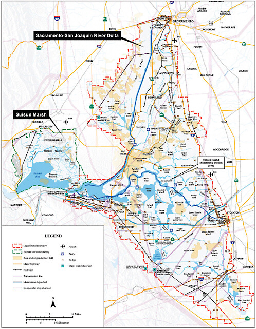
only be determined for, a given location. Two examples of coastal impacts are discussed here: New York City and the Sacramento-San Joaquin Delta of California.
New York City (NYC) is both a mega-delta and a mega-city located along the eastern seaboard of the United States. Return times of current 100-year and 50-year coastal storms for NYC are strongly correlated with global and local sea level rise (Figure 5.10, based on Kirshen et al., 2008a). Based on historical records, the projected frequency of coastal storms can be translated into an estimate of the number of buildings in downtown NYC that would be damaged by storms characterized by their current FEMA-based return times (Figure 5.11, based on NYCOEM, 2009).
New York City has responded to these risks by considering a range of adaptation options to reduce the vulnerability of its critical public and private infrastructure over time (NPCC, 2009). One option envisions creating a dynamic process by which FEMA systematically redraws its 100-year flood maps as sea level rises, so insurance markets could appropriately spread the risk. Other plans envision constructing retractable barricades to protect New York from an impending storm—much like the barrage on the Thames that protects London (where plans are underway to build a new barrier based on observed and estimated sea level rise); the barrier that protects St. Petersburg, Russia; and multiple devices now being installed to protect Venice at the border of its lagoon and the Adriatic Sea. The city is considering adjust-
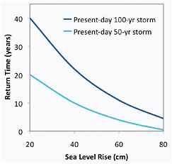
FIGURE 5.10 Projected return time of coastal storms relative to future sea level rise for New York City (Based on Kirshen et al., 2008a).
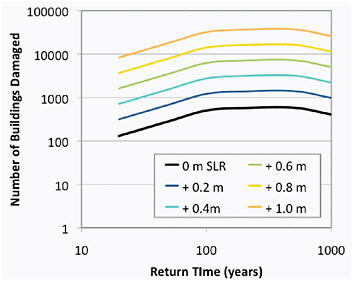
FIGURE 5.11 Expected number of buildings that would be damaged in the present-day downtown New York City, for various types of storms for different sea level trajectories. Based on information presented in Figure 5.10 that includes more detail for intermediate return times and damage estimates from NYCOEM (2009).
ments in building codes and zoning regulations designed to maintain the specific “climate (risk) protection levels” embedded in existing legislation and operating procedures.
On west coast of the United States, the Sacramento-San Joaquin Delta region is home to farms, roads, oil and gas lines, and extensive housing developments (Figure 5.12). The entire Delta is below mean water level, much of it more than 15 feet below. The magnitude of impacts from sea level rise and storm surge breaching of the levees currently protecting the region is estimated at tens of billions of dollars over the next few decades alone (CALFED, 2009).
The California Bay-Delta Authority is exploring options to divert large amounts of water away from the region and/or cut losses in certain areas by deciding ahead of time what to replace and what to leave. Other regions, such as the metropolitan Boston area, have also identified areas likely to flood, and they are exploring the efficacy of prevention and adaptation options such as preserving coastal wetlands and relocating water treatment plants away from the coasts (Kirshen et al., 2008a).
Transportation, Buildings, and Structures
Impacts on transportation and built structures are primarily the result of changes in temperature and precipitation beyond what the materials used to build the roads, rails, bridges, and buildings were designed to withstand. Transportation can also be impacted by extreme temperatures, heavy rainfall events, and persistent freeze/thaw conditions.
Climate patterns based on the past century, traditionally used by transportation planners to guide their operations and investments, may no longer provide a reliable guide to the future (NRC, 2008). In many northern cities, for example, standard building procedures do not require air conditioning. As temperatures increase, many of these may require expensive retrofits so they can continue to be used in extreme heat.
Across the United States, the average number of days per year with very heavy precipitation has increased significantly over the past 50 years, with the largest increases (58 and 27 percent, respectively) occurring in the Northeast and Midwest regions (USGCRP, 2009). This trend is expected to continue in the future across many regions, as extreme precipitation events increase (Tebaldi et al., 2006). In both the Midwest and Northeast, climate change is also expected to increase the amount of rain that falls in winter and spring, when frozen and/or saturated ground increases flood risk, while decreasing summer and autumn rainfall (Hayhoe et al., 2008, 2010). Increased frequency of winter and spring rainfall, combined with more frequent precipitation extremes, could lead to higher peak stream-flows, particularly under higher temperature change and toward the end of the century (Cherkauer et al., 2010). Infrastructure impacts in Chicago are highlighted in Box 5.3.
Energy
Climate change is likely to affect energy demand, production, and reliability (Wilbanks et al., 2007). Although warmer winter temperatures are expected to reduce demand for heating energy, observed correlations between daily mean near-surface air temperature and electricity demand suggest that warmer summer temperatures and more frequent, severe, and prolonged extreme heat events will likely increase demand for cooling energy, particularly as use of air conditioning increases around the world (see Figure 5.14).
The impact of increasing temperatures on air conditioning demand could have a disproportionately large effect in already heavily air-conditioned
|
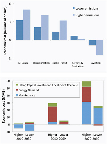
BOX 5.3 INFRASTRUCTURE IMPACTS IN CHICAGO One of the few detailed analysis of potential economic costs of a range of climate change scenarios for transportation infrastructure has been conducted for the city of Chicago (Hayhoe et al., 2010). Chicago has experienced impacts from weather extremes, when city streets buckled and rail lines warped during the record-breaking 1995 heat wave; or in 1996, when 17 inches of rain fell in a single 24-hour period, with a total estimated cost of flood losses and recovery of $645 million (Changnon et al., 1999). Impacts of changes in mean and extreme temperature and precipitation on Chicago’s public transit, maintenance and construction of roads, highways, bridges, and canals, and airport operations are estimated at $3.3 million under an approximate 2ºC change in global mean temperature and $5 million under a 4ºC change (Figure 5.13a). Estimates for building-related expenses under higher temperature change are likely to be 10 times greater (conservatively $20 million) than under lower (Figure 5.13b). Values are based on only the sensitivities city officials were aware of based on past conditions and events. |
regions, such as the Southwest (Miller et al., 2008). Projected increases in peak electricity demand in particular raise concerns regarding electricity shortages, as risk of shortages may increase with both mean and extreme temperatures.
Electricity generation by fossil and nuclear power plants requires a large supply of water, which may become limited during periods of drought. Although thermoelectric power plants in the United States have not yet had to reduce operations due to insufficient water supply, future water shortages are expected to affect power production in a number of states (Wilbanks et al., 2007). The reliability of energy supplies can be affected by the frequency of droughts and accompanying heat waves, which increase the temperature of the cooling water beyond what the plant may be permitted to release.
Hydropower, which accounts for 75% of renewable power generation in the United States and the majority of all electricity supply for many nations in South America and Northern Europe, is the most directly sensitive to water availability. The relationship between hydropower generation and precipitation tends to be proportional, with a 1% change in precipitation resulting in approximately 1% change in power generation. However, projecting future climate effects on hydropower generation is limited by uncertainties in precipitation projections. For example, recent projections of hydropower generation in the Sierra Nevada Mountains of California ranged from –10% to +10%, depending on the climate model used (Vicuña et al., 2008). Similarly, projections for the Pacific Northwest ranged from +2% to –30%, depending on the precipitation projections (Markoff et al., 2008).
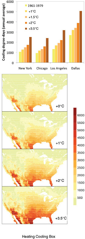
FIGURE 5.14 Heating/cooling degree-days. Projected changes in heating and cooling degree-days for: (a) four U.S. cities by global temperature change, and for (b) the continental United States (Based on USGCRP, 2009). A first approximation for heating and cooling demand is provided by estimates of projected changes in heating and cooling degree-days (Rosenthal et al., 1995; Amato et al., 2005). Projections of the increase in cooling energy use range from 5% to 20% per 1ºC increase in temperature for residential buildings and about 9 to 15% per 1ºC for commercial buildings. The relationship between cooling energy demand and temperature is nonlinear, with greater increases in demand occurring at higher temperatures (Wilbanks et al., 2007).
5.6
HEALTH
Increasing temperatures alter the risk of direct and indirect weather-related impacts on human health, from cardiovascular and respiratory illnesses to infectious diseases (Patz et al., 2005). Quantifying the impact per degree of global temperature change, however, is complicated by confounding factors such as human behavior and socioeconomic conditions that affect exposure, transmission, and other aspects of risk (Patz et al., 2005). Here, we discuss three main aspects of health-related risks likely to be affected by climate change: heat-related illness and death, vector-borne disease, and health concerns related to poor air and water quality.
Heat-Related Illness and Death
Temperature extremes such as heat waves and periods of extreme cold are known to produce elevated rates of illness and death (McGeehin and Mirabelli, 2001). Together, these accounted for 75% of all deaths due to natural disasters from 1979-2004 (Thacker et al., 2008). From the 1970s through the 1990s, heat-related mortality in the United States declined due to acclimatization and increased use of air conditioning, then flattened out during the past decade (Sheridan et al., 2009).
In the future, extreme heat days and heat wave frequency, intensity, and duration is projected to increase with global mean temperature, while the frequency and intensity of winter cold is projected to decrease (Tebaldi et al., 2006; IPCC, 2007a). Under a 2ºC increase in global mean temperature by end-of-century, for example, the average number of days per year with maximum temperatures exceeding 38ºC or 100ºF across much of the south and central United States is projected to increase by a factor of 3. Under a 3.5ºC increase, the number of days is projected to increase by 5 to nearly 10 times historical levels (Figure 5.15).
Although the response of illness and death rates to changing heat extremes can be modified by acclimatization and adaptation strategies (Ebi et al., 2004), it is clear that risks of heat-related mortality increase with temperature, while cold-related mortality risks decrease (Gamble et al., 2008). Prolonged periods of extreme heat with little relief at night can have devastating effects on urban populations (Basu and Samet, 2002), increasing the risk of both illness and death due to heat stress (Martens, 1998; McGeehin and Mirabelli, 2001; Schär et al., 2004).
Temperature-related mortality is strongly linked to a wide variety of social, economic, and behavioral factors, even in industrialized nations such
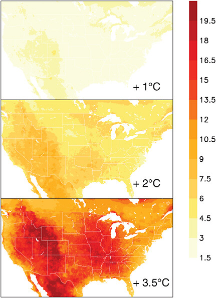
FIGURE 5.15 Projected increase in heat wave duration index, in number of days per event. Defined after Frich et al. (2002) and Tebaldi et al. (2006) as the longest period each year with at least 5 consecutive days during which daily maximum temperature is at least 5ºC higher than the climatological (1961-1990) average for that same calendar day. Projected changes are for 20-year periods during which mean global mean temperature increased by 1ºC, 2ºC, and 3.5ºC, respectively relative to the 1961-1979 average.
|
BOX 5.4 HEAT-RELATED MORTALITY IN CHICAGO The Chicago heat wave of 1995 is estimated to have been responsible for 692 heat-related deaths within the city of Chicago itself (Kaiser et al., 2007). As global mean temperatures increase, 1995-like conditions are projected to become more frequent in Chicago. Under a 2ºC change in global mean temperature, annual average mortality rates are projected to equal those of 1995. Under a 4ºC change in global mean temperature, annual average mortality is projected to be twice 1995 levels, with 1995-like heat waves occurring as frequently as three times per year (Hayhoe et al., 2010). |
as the United States (e.g., Basu, 2009; Ekamper et al., 2009). Since observed mortality rates are more responsive to changes in high temperature than low temperature extremes, at the global scale an overall increase in heat-related deaths is expected to exceed the projected decrease in cold-related deaths (Medina-Roman and Schwartz, 2007).
Several recent severe heat waves have focused public attention on the health risks associated with extreme heat, including a 1995 heat wave in Chicago (see Box 5.4) and the unprecedented European heat wave of 2003, estimated to be responsible for approximately 70,000 excess deaths across 16 European countries (Robine et al., 2008). Past events such as these can be used as case studies for evaluating the potential impacts of future climate conditions. For example, observations of the health effects of a heat wave in California in July 2006 showed that heat-related mortality increased 9% for every 5.5ºC increase in apparent temperature, with that specific event causing an estimated 160-505 deaths, a 6-fold increase in the number of heat-related visits to the emergency room, and 10-fold increase in heat-related hospitalizations (Knowlton et al., 2009; Ostro et al., 2009).
Using an analogue approach, Kalkstein et al. (2008) estimated the number of heat-related deaths that might occur in U.S. cities if they experienced conditions similar to the severe Paris heat wave of 2003. Compared to the hottest summers on record, heat-related deaths in St. Louis and New York are projected to increase by 29% and 155%, respectively. Other cities, including Washington, Philadelphia, and Detroit, could experience 2-11% more heat-related deaths, compared to their hottest summers on record. This range of response illustrates the variation among cities in their sensitivity to extreme heat, which might result from factors such as baseline climate conditions (cooler cities may be more susceptible to heat), demographic patterns, and acclimatization measures such as air conditioning.
Heat watch-warning systems presently in operation in major U.S.,
Italian, and Canadian cities have already been shown to save a number of lives when coupled with effective intervention plans (Ebi et al., 2004). These systems, coupled with well-developed intervention activities, represent an important way to lessen the potential for drastic increases in heat-related mortality in coming decades due to climate change.
Long-Term Impacts of Heat Stress
Many of the impact studies summarized in this section and elsewhere throughout this report focus on future projections for the next few decades; nearly all of the impact studies in the literature, regardless of focus area, confine estimates of potential impacts to this century. This limits quantification of impacts based on GCM simulations driven by the SRES scenarios to those associated to global mean temperature changes of 4ºC or less, depending on the GCMs and scenarios used to generate future projections.
One recent study, however, attempts to extrapolate beyond this threshold by using long-term simulations reaching a global temperature change of 10ºC relative to 1999-2008 (Sherwood and Huber, 2010). Recognizing that most of the impacts studied to date depend on assumptions about future conditions that cannot be reliably simulated with our current state of knowledge, the authors instead focus on an impact that depends on a basic physiological threshold: specifically, that associated with the need of the human body to dissipate the heat it generates. This can happen only if the temperature to which the skin is exposed is lower than the skin temperature itself.
The authors consider future statistics of annual maximum wet bulb temperatures exceeding average human skin temperature of 35ºC as a measure of heat stress on humans and other mammals, and illustrate how, assuming carbon emissions and climate change continue unchecked beyond this century, the magnitude of land area that could become uninhabitable due to heat stress could be greater than that lost to sea level rise over the same time frame. Although exact projections of changes in inhabitable land area over multiple centuries are sensitive to key uncertainties in carbon cycle, climate sensitivity, and ocean-atmosphere dynamics discussed in Chapters 3 and 4, this study raises an important point: namely, that hard-wired, physiological limitations on human welfare have not previously been acknowledged in evaluating the long-term risks associated with a given pathway of carbon emissions.
Pests and Disease
Changes in climate can affect the spread of illness and diseases such as malaria and West Nile Virus, carried by animal hosts and mosquito, midge, fly, or tick vectors. Increasing temperatures and changes in precipitation patterns can accelerate current trends of increased risk of exposure to disease by expanding the geographic range and/or populations of the vectors (Ogden et al., 2008). In addition to the potential for more vectors to be present, warmer temperatures increase the virus replication rate, increasing the efficiency of virus transmission (Mellor, 2000).
Despite initial projections suggesting the potential for dramatic future increases in the geographic range of malaria and other infectious diseases under climate change (e.g., Martin and Lefebvre, 1995), subsequent studies have highlighted how the complexity of the systems—involving viral, bacterial, plant, and animal physiology, as well as sensitivity to changes in climate extremes, including precipitation intensity and temperature variability—challenges attempts to resolve the influence of historical climate change on observed trends in disease incidence and develop future projections specific to any particular level of global temperature change. This is even true for what many previously considered the poster child for the influence of climate change on infectious diseases, the spread of malaria throughout the East African highlands (e.g., Pascual et al., 2006).
If historical contributions are difficult to resolve, prediction of future trends is even more so. Most recent projections suggest that the ranges of malaria and other diseases may shift, but increases in some areas will likely be balanced out by decreases in others, resulting in little net increase in area (Lafferty, 2009). The potential for genetic mutation, the influence of changing agricultural techniques, and increased transportation and trade between regions previously not in regular contact are all confounding factors that have been cited as complicating the influence of climate change on a given disease (Gould and Higgs, 2009).
It is also important to remember that good sanitation and insect control programs can limit disease spread even under suitable climate conditions (Lafferty, 2009). In 1882, malaria in the continental United States extended from the Gulf of Mexico to Minnesota. Draining of swamps, improved pesticides, and better management of water resources contributed to the eradication of malaria in the United States shortly after World War II (Oaks et al., 1991). Replicating methods proven successful in the past may be one way to reduce the risk associated with climate change and vector-borne disease.
Air and Water Quality
Increasing temperatures and changing precipitation intensity can also affect air and water quality. Densely populated areas with warm summers tend to have high levels of ozone precursor emissions (nitrogen oxides and volatile organic compounds). These precursor species react in the presence of sunlight, with key reactions proceeding faster at higher temperatures. Ground-level ozone, the primary component of smog, is a respiratory irritant that decreases lung function and may increase the development of asthma in children (Tagaris et al., 2009).
In the future, warmer temperatures and changes in atmospheric circulation patterns may bring oppressive summer weather patterns earlier in the year (see Section 4.4), accelerating the formation rates of tropospheric ozone and increasing the length of time photochemical smog remains over any given location. Barring significant decreases in precursor emissions, tropospheric ozone exceedences could become more common over most densely populated areas in the United States, China, and elsewhere around the world with warm summers (Mickley et al., 2004; Tao et al., 2007; Lin et al., 2008). A study of 50 U.S. cities projected that a 1.6 to 3.2ºC increase in local temperature would lead to an average 4.8 ppb increase in ozone levels by 2050, with the greatest increases occurring in cities with already high ozone concentrations (Bell et al., 2007). Ozone levels were projected to exceed the 8-hour regulatory standard an average of 5.5 more days per summer, an increase of 68% over current conditions. Although ozone mortality was projected to increase by 0.11 to 0.27% on average, certain cities exhibited greater sensitivities (e.g., increases of 5% for New York City; Knowlton et al., 2008). Given the sensitivity of ozone levels to precursor emissions, climate effects on ground-level ozone and particulate matter may depend less on direct temperature effects and more on the effectiveness of pollution control measures and climate-driven changes in natural emissions sources (Ebi and McGregor, 2008).
Increasing frequency of heavy downpours is already occuring and is projected to continue to occur in many parts of the world, including the eastern United States (Tebaldi et al., 2006; Karl et al., 2009). These increase the risk of water contamination and spread of water-borne bacterial diseases, with the risk being exacerbated by rising temperatures (Vorosmarty et al., 2000). Current and future deficiencies in watershed protection, infrastructure, and storm drainage systems will likely increase the risk of contamination events as climate variability increases (Rose et al., 2000).
The length of the pollen season has already increased due to both earlier onset of flowering (Parmesan, 2007) and lengthening of the season for late-
flowering species (Sherry et al., 2007). In the future, increasing temperatures may also affect the production, toxicity, and/or pollen-producing capacity of allergenic and toxic plants, including ragweed and poison ivy (Mohan et al., 2008; Shea et al., 2008; Ziska et al., 2009). Allergy incidence may also be increased by interactions between airborne allergens and air pollution (D’Amato and Cecchi, 2008). Uncertainties in future emissions and the coupling between climate, air quality, and ecosystem models, however, render speculative any determination of the degree of change (Bernard and Ebi, 2001; Gamble et al., 2008).
5.7
ECOLOGY AND ECOSYSTEMS
Terrestrial Species and Climate Change: What Species Are Up Against
As the climate changed throughout the past millennia, species shifted to track temperature, precipitation, and other weather factors (Graham and Grimm, 1990; Overpeck et al., 1992). The geographic range of any species includes only areas where individuals can endure the extreme temperature and water stress occurring at those locations (Gordon,1982; Chown and Gaston, 1999). Indeed, the ranges of various songbirds in North America are limited by the amount of metabolic energy an individual must exert to stay alive (Root, 1988a,b). Warming in the late-Quaternary resulting in species tracking the changing climate gradient (Graham and Grimm, 1990). Additionally, these species differentially tracked their own unique set of climatic factors, which resulted in many species occurring in unexpected areas (Graham and Grimm, 1990) and new species groups being formed (Overpeck et al., 1992; Hobbs et al., 2009).
Today species continue to shift and change with current climate change. Additionally, if we remain on the “Business as Usual” scenario, then on a sustained global basis the expected rate of change in temperature in the next few decades could be higher than most species have endured over millennia (Hoeg-Guldberg et al., 2007; Loarie et al., 2009; NRC, 2009). In addition the face of the planet is very different from how it has ever been before because people have altered it considerably by constructing various structures on the landscape, such as cities, farms, and roadways. These frequently make movement of species across an area difficult. This is particularly true for species that are slow moving, such as turtles, but it is also true for animals that can move more quickly, including birds, bats, and butterflies. Even with these impediments, many species are changing with the globally changing climate. Indeed, with an increase in the average global
temperature of only ~0.6ºC, many species around the globe were found to be making many significant changes (Root and Schneider, 2002; Parmesan and Yohe, 2003; Root et al., 2003). Species primarily exhibit two different types of changes: the timing of various temperature-related events, such as blooming or egg laying; and shifting their ranges to formerly cooler regions, such as poleward and up in elevation for terrestrial species and descending deeper in the oceans for marine species (Root and Schneider, 2002; Parmesan and Yohe, 2003; Root et al., 2003; Root et al., 2005; Parmesan, 2006; Fox et al., 2009). Species are exhibiting other types of changes, but they are not reported as often as these two changes. Included in this “other” category are, for example, behavioral changes, changes in size and shape, and genetic changes.
Change in Seasonal Timing
The timing of different seasonal activities (phenology) of many species is shifting in concert with the changing climate. Common changes in the timing of spring activities include the timing of migration in various species such as birds, mammals, fish, and insect species (e.g., MacMynowski and Root, 2007; Ogden et al., 2008) and in budding, blooming, and leafing in plants (e.g., Menzel et al., 2006; Crimmins et al., 2009; Primack and Miller-Rushing, 2009). For example, in the case of plants, several trees in an urban to rural setting in Ohio exhibited an earlier trend in the leafing out in the spring (Shustack et al., 2009). The same is true for the timing of cherry blossoms in Japan, for which data exist from the ninth century (Primack et al., 2009). Satellite data unequivocally confirm the earlier greening of the biosphere (Myneni et al., 1998; White et al., 2009). Of course individual examples are not sufficient to draw generalized conclusions, thus meta-analyses have been performed to look for consistent patterns around the globe over a large number of species that have been observed to have been changing. For all Northern Hemisphere species reported in the literature with more than a 10 year record showing phenological changes in the spring, the average number of days changed in the spring observed over the last 30 years of the 20th century was ~15.5 days or ~5 days per decade earlier timing for those species showing a phenological change in the spring (Root et al., 2003). When both the species changing and those not changing in the same areas are included in the study calculation, then the number of days drops strongly to ~2 days per decade (Parmesan and Yohe, 2003). The increase in global average temperatures over that time period was ~0.4ºC, although changes in land temperatures, especially at higher latitudes, were some factor of two larger (IPCC, 2007a).
Contrary to what has been found for spring phenology, trends in autumn phenologies are not as clear. In the spring, animals are getting ready to breed and are driven to breed as earlier as possible. Therefore, these species arrive earlier as the springtime warms, which in turn means they need earlier availability of required resources such as food. If a needed resource is not shifting in concert with a species exhibiting shifts, this could cause some decline in breeding success, for example. In the autumn some leaf fall is delayed, and some migrating animals move their southern migration date earlier than it was before, while others migrate south at roughly the same time that they always have migrated, and some stay longer before migrating (Miholcsa et al., 2009; Schummer et al., 2010).
Mismatch in Timing
Over evolutionary time species have formed predator-prey relationships that are being disrupted because the predator and prey do not necessarily respond to warming by shifting in concert. For example, the common cuckoo (Cuculus canorus), a migrant, is a brood parasite laying its eggs in the nests of other birds that migrate either short or long distances. With climate change the short-distance migrants are arriving significantly earlier now than in the past and they are nesting before the cuckoo has arrived. Consequently, the short-distant migrants have reduced brood parasitism (Saino et al., 2009). This is an example where there are both winners and losers with climate change—the short-distance migrants winning and the cuckoo losing. What is “better” or “worse” is of course a value judgment, yet if one species is aided whereas others are disadvantaged to the point of population collapses and perhaps extinction, then the net effect could mean a local loss of species.
Range Shifts
As the climate has changed species have shifted their range because they are attempting to stay in areas where they are exposed to the same regional ambient temperatures. For terrestrial species this means moving toward the pole and up in elevation. From 1914 to 1920, Joseph Grinnell systematically surveyed a 60 to 3,300 m elevation gradient in Yosemite National Park. He kept meticulous field notebooks, and these have been valuable in studying changes in species over a century, because the same area was resurveyed from 2003-2006. Roughly half of the 28 mammals surveyed moved up in elevation by an average of around 500 m. For example, one of the species shifting up in elevation in response to climatic warming is the
American pika (Ochotona princeps) (Moritz et al., 2008). In 1917 Grinnell found it up to 2,400 m (Grinnel, 1917), but in 2004 it was recorded up to 2,900 m. The same type of analysis with similar results has also been done on birds (Tingley et al., 2009). Changes in the species are consistent with an increase in minimum January temperature by about 3ºC.
In prehistoric times many species communities were composed of species that today are not found together (Overpeck et al., 1992). These so-called no analog communities foreshadowed what we are now observing; many species are moving differentially, which means the various biotic interactions existing within some species communities are changing. For example, the predator-prey cycle will be broken if one species moves into areas where the other does not occur. A situation that could cause concern is if the prey is a pest on our crops or a disease vector, and they no longer are held in check by the predator. Even if mutalistic interactions are disrupted, such as an insect that commonly pollinates a crop shifts, another insect pollinator most likely will move in, but perhaps not immediately. In several locations around China people are having to hand pollinate apple and pear trees to counter the loss of productivity due to a significant decline in the abundance of natural pollinators (Partap et al., 2001).
Changes in Size and Shape, Genetics, and Behavior,
As Earth has warmed many species are showing different types of concurrent changes. Hadly (1997) documented body size changes of a small mammal during historical (natural) climate shifts. Temporal fluctuations of body size in woodrats are so precise that Smith and Betancourt (1998) labeled them “paleo-thermometers.” Indeed, two rodent species in southern New Mexico captured from 1991 to 1998 had multiple structures, such as hind leg, ear, and body length, showing strong correlation with a time-appropriate climate variable (Wolf et al., 2009).
Few studies have found a change in genetics with climate change. This could be that relatively few scientists have looked for such a change. Bradshaw and Holzapfel (2008), however, have examined the pitcher-plant mosquito (Wyeomyia smithii), and they did find genetic change (Bradshaw et al., 2006).
Species most affected by reductions in Arctic sea-ice extent are those with limited distributions and specialized feeding habits that depend on ice for foraging, reproduction, and predator avoidance, including the ivory gull (Pagophila eburnean), Pacific walrus (Odobenus rosmarus divergens), ringed seal, hooded seal (Cystophora cristata), narwhal (Monodon monoceros), and polar bear (Ursus maritimus); see Post et al. (2009) and Gilg et al. (2009).
Synergetic Forces
Given the changes humans have made to the planet, many more factors than climate change are affecting species (Laurance and Useche, 2009). These include such things as land-use change, invasive species, introduced chemicals, and hunting. Additionally, changes to a system can feedback on other systems, which in turn may cause species more stress, for example, loss of coastal marshes causing increased erosion. Managers have been working for decades to help species combat stresses, for example, by setting up refuges for ducks where they are provided artificial lakes, food, and hunting protection. Coping with one or even two of these stresses can be difficult for species, but now adding the ubiquitous stress of a changing climate has managers and others concerned about possible population declines, and in extreme cases, extinction.
Certain traits can make a species more prone to extinction. These include the size of the species population (large population size is much more stable than a small size); the size of the range of the species (a species with a larger range size is less likely to become rare and then extinct); and species that specialize on a particular trait, such as a particular prey item or a particular tree for nesting. In the last case, such dependent species are at greater risk of extinction due to their reliance on a particular item that could itself be negatively changed by climate change. Such change can actually cause a cascade of changes through the species communities due to the interconnectedness experienced by species within an ecosystem.
Extinction
The average lifespan of a plant or animal species is ~7 million years, which is the number of years a species persists from when the species arises via speciation to when it goes extinct (Lawton and May, 1995). The best estimate of how many plants and animals are extant compared to all plants and animals that have ever existed is around 2%. Consequently extinction is certainly a normal occurrence. The background level of extinctions (not human induced) differs with different taxa and types of species. In marine species it is estimated to be ~0.1 to 1 Extinction per Million Species Years (E/MSY). The number for mammals is similar, being ~0.2-0.5 E/MSY (Foote, 1997; Alroy, 1998; Regan et al., 2001; MEA, 2005; May, 2010).
Determining historic extinction rates is difficult because of the time it takes for a species committed to extinction—extinction will occur without some major change occurring, such as human management—to reach the point when we can document that the individuals in the population are no
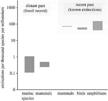
FIGURE 5.16 Species extinction rates, expressed as extinctions per 1,000 species per 1,000 years. The fossil record tells us that in the distant past less than one mammal went extinct every 1,000 years. In the recent past the number of extinctions has increased 3 orders of magnitude higher than that of the fossil record. SOURCE: May (2010).
longer replacing themselves. These species are called functionally extinct. When that assistance is not possible, there is still a time lag due to humans not being comfortable declaring a species extinct. Indeed, there is a “50-year rule” that says a species cannot be said to be extinct until it has not been found for 50 years. Even so, current rates of extinctions can be calculated at least for well-studied species, i.e., mammals, birds. and amphibians. The number of species in these three taxa is around 21,000, and over the past century ~100 species in those taxa are known to have gone extinct, giving an extinction rate of ~50 E/MSY (MEA, 2005). Adding the functionally extinct species, the rate of “extinction” increases to ~200 (May, 2010; see Figure 5.16).
What about future extinctions? For many decades now we have known the importance of three factors in contributing to a species becoming a concern with regard to extinction (Rabinowitz et al., 1986): (1) The overall range size is small enough for a major perturbation to influence greatly all
individuals in the species (Harris and Pimm, 2008). For example, the whooping cranes (Grus americana) while on their wintering ground in Texas are at high risk if there is an oil spill or powerful hurricane because the entire population winters in a small inlet along the coast; (2) The overall population size is small, which can be detrimental because breeding in a small population can result in inbreeding (Liao and Reed, 2009). This, in turn, can increase the expression of deleterious genes, which decreases the number of fit young being produced, and the loss of genetic variability, which is needed to allow adaptation to novel habitats; and (3) The population depends on some factor or species that could be at risk from disturbances, such as pollution, poaching, or climate change, among others. For example, the red-cocked woodpecker (Picoides borealis) must nest in 70- to 120-year-old pines, most of which in the late 1800s and mid 1900s were cut down for various uses. Another example involves plant-eating insects, of which there are estimated to be 213,830 to 547,500 species committed to extinction because the range of their host plants are shrinking in size because of warming (Fonseca, 2009).
When climate change is one of the main forces acting on a species, then distance to closest cool refuge (Figure 5.17) is also as important as
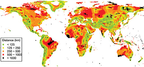
FIGURE 5.17 Map showing the distance to potential cool refuges, where cool is defined as the temperatures in 2100 are equal to or cooler than the temperatures in the 1960s. Used 0.5 x 0.5 latitude-longitude blocks. Source: Wright et al. (2009).
range size, population size, and the vulnerability of a population depending on some limited factor at risk. Reaching the cool refuge is crucial. For example, Sinervo et al. (2010) reported lizards, which have body temperatures determined by habitat temperatures, on four different continents are having to spend more time than before escaping warming temperatures by going into burrows or other locally cooler places. This means they have less time to forage and hence do not have the energy reserves needed to successfully reproduce, which of course can lead to population decline and possibly extinction. These species and others could probably avoid extinction by moving into new other areas in the region that are cooler (e.g., up in elevation). If a species in question has a maximum dispersal distance that is shorter than the distance to the refuge, or if the species is not a good colonizer and fails to become established in the refuge once it gets there, then the species will be in trouble unless it gets human assistance. Species that are in trouble unless aided by humans are called functionally extinct. Examples of functionally extinct species are those that are on oceanic islands or mainland islands, such as oasis within a desert, because unless they fly, dispersing to a cooler refuge is not possible. For example, the Akiapolaau (Hemignathus munroi) on the Hawaiian Islands, Aruba island rattlesnake (Crotalus durissus unicolor), and the black robin (Petroica traverse) on Chatham Islands off the coast of New Zealand are all critically endangered and will go extinct without help from humans.
Hubbell and co-workers (2008) looked at possible extinction rate in the Brazilian Amazon due to land-use change. He estimated that a total of 11,210 tree species occur in the Brazilian Amazon. About 30% of these trees (~3,250) have populations greater that 1 million, and consequently, do not currently face extinction. Fifty percent (~5,300) of all the species have populations less than 10,000. Roughly 35% of these have a high probability of going extinct even without the effects of climate change. This would also result in insects and other species that depend on these tree species to also be facing extinction. Climate change and other drivers could exacerbate the vulnerability of these species of concern.
Deutsch and co-authors (2008) investigated the physiological tolerances of species from pole to pole. They found, as expected, that the extent of physiological tolerance was wider at the higher latitudes and narrower near the equator. From this they reasoned that the tropical species could very well have a more difficult time as the globe warms, because the temperature to be experienced by species in the tropics could well be higher than that ever experienced by the tropical species. Temperate, boreal, and arctic species will also be subjected to warmer temperatures, but those temperatures, for
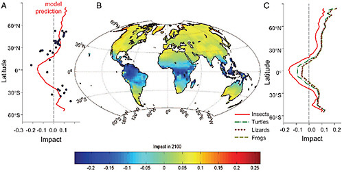
FIGURE 5.18 Predicted impact of warming on the performance of animals with body temperatures equilibrated to ambient (ectothermic or cold-blooded). On both panels the red line is the model output. On the right panel the dots are the intrinsic growth rates for each insect species examined. On the left panel other terrestrial ectotherms, including frogs, toads, lizards, and turtles are plotted. Source: Deutsch et al. (2008).
a while at least, will be within the variability of temperatures experienced. Hence, tropical trees, and other studies will highly likely find the same to be true for tropical animals and are at higher risk of not being resilient to the incipient warming (Figure 5.18).
Using the A1B scenario from IPCC (2007a), Wright and co-authors (2009) found that “75% of the tropical forests present in 2000 will experience mean annual temperatures in 2100 that are greater than the highest mean annual temperature that supports closed-canopy forest today” (p. 1418). As long as there is a cool refuge within dispersal distance and as long as dispersal is possible this increase may not be a big problem. The most common cool refuges for plants are to migrate up in elevation. In the tropics, however, such elevational relief is not available, making cooler refuges for many plants and animals living in the tropics inaccessible. Around 1,200 mammals have ranges restricted to the low-latitude tropics with no easy access to cooler refuges as the globe warms. Another group of mammals at risk of extinction are those about 650 species that have ranges smaller than
3,130 km2. Without aid from humans these species are probably not going to be able to persist.
Extinction is irreversible. Choices among stabilization targets can be expected to determine the scope of future extinction (e.g., types of species, geographic regions, etc.) that could be caused by climate change, or alternatively the scale of protective adaptation measures such as species management that could be considered to avoid extinctions.
5.8
BIOLOGICAL OCEAN
Impacts of CO2, pH, and Climate Change in the Ocean’s Biology
Marine ecosystems will be affected by climate change via physical changes in ocean properties and circulation (Sections 4.1, 4.4, and 4.7), ocean acidification via altered seawater chemistry from rising atmospheric CO2 (Section 4.9), and sea-level rise via coastal habitat loss. Some of the key potential impacts will involve changes in the magnitude and geographical patterns of ecological and biogeochemical rates and shifts in the ranges of biological species and community structure (Boyd and Doney, 2002). Impacts are expected to include both direct physiological impacts on organisms through, for example, altered temperature, CO2, and nutrient supply, and indirect effects through altered food-web interactions such as changing seasonal timing (phenology) of phytoplankton blooms or disruptions in predatory-prey interactions.
Primary production by upper-ocean phytoplankton forms the base of the marine food-web and drives ocean biogeochemistry through the export flux of organic matter and calcareous and siliceous biominerals from planktonic shells. Plankton growth rates for individual species are temperature dependent and tend to increase under warming up to some threshold. When viewed in aggregate, plankton community production rates approximately follow an exponential curve in nutrient replete conditions, which would suggest increasing global primary productivity over this century as sea surface temperatures increase (Sarmiento et al., 2004). In most regions of the ocean, however, primary production rates are limited by nutrients such as nitrogen, phosphorus, and iron. Diatoms, a key shell-forming group of phytoplankton, are also limited by silicon. The rates of many other biological processes, such as bacterial respiration and zooplankton growth and respiration, also speed-up as temperature rises, the integrated effect at the ecosystem level is difficult to predict from first principles. Warming also occurs in conjunction
with other factors (rising CO2, altered ocean circulation), and the potential synergistic or antagonistic effects of multiple stressors must be considered.
Satellite observations indicate a strong negative relationship, at interannual time scales, between marine primary productivity and surface warming in the tropics and subtropics, most likely due to reduced nutrient supply from increased vertical stratification (Behrenfeld et al., 2006). Satellite data also indicate that the very lowest productivity regions in subtropical gyres expanded in area over the past decade (Polovina et al., 2008), although these trends may be due to interannual variability (Henson et al., 2010). Numerical models project declining low-latitude marine primary production in response to 21st century climate warming (Sarmiento et al., 2004; Steinacher et al., 2010) (Figure 5.19). Warmer, more nutrient-poor conditions in the subtropics could enhance biological nitrogen fixation (Boyd and Doney, 2002), an effect that may be amplified by higher surface water CO2 levels (Hutchins et al., 2009). The situation is less clear in temperate and polar waters, although there is a tendency in most models for increased production due to warming, reduced vertical mixing, and reduced sea-ice cover. For example, the rapid warming and sea-ice retreat along the West Antarctic Peninsula has lead to a poleward shift in the region of strong seasonal primary production that has impacts for higher trophic levels including seabirds (Montes-Hugo et al., 2009). In most open-ocean regions, however, the climate signal in primary production and other ecosystem properties may be difficult to distinguish from natural variability for many decades (Boyd et al., 2008; Henson et al., 2010). Changes in atmospheric nutrient deposition (nitrogen and iron) linked to fossil-fuel combustion and agriculture also can alter marine productivity but mostly on regional scales near industrial and agricultural sources (Duce et al., 2008; Krishnamurthy et al., 2009).
Subsurface oxygen levels likely will decline due to warmer waters (lower oxygen solubility) and altered ocean circulation, leading to an enlargement of open-ocean oxygen minimum zones and stronger coastal oxygen depletion in some regions (Keeling et al., 2010; Rabalais et al., 2010). Low subsurface O2, termed hypoxia, occurs naturally in open-ocean and coastal environments from a combination of weak ventilation and/or strong organic matter degradation. Dissolved O2 gas is essential for aerobic respiration, and low O2 levels negatively affect the physiology of higher animals leading to so-called “dead-zones” where many macro-fauna are absent. Coastal hypoxia can lead to marine habitat degradation and, in extreme cases, extensive fish and invertebrate mortality (Levin et al., 2009; Rabalais et al., 2010). Expanded open-ocean oxygen minimum zones would increase denitrification and may contribute to increased oceanic production of the greenhouse gas
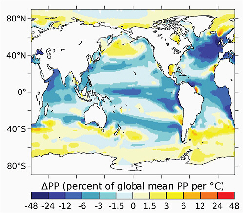
FIGURE 5.19 Model projected change in vertically integrated annual mean primary production (PP) relative to pre-industrial conditions (decadal mean 1860-1869) for the end of the 21st century under SRES A2. The changes represent the difference between 2090-2099 and 1860-1869 (decadal means). Multi-model means have been computed for four coupled ocean-atmosphere models using regional skill scores as weights. Where no observation-based data is available to calculate skill scores (e.g., in the Arctic) the arithmetic mean of the model results is shown. The magnitude of the primary production changes are shown in percent normalized to global mean areal primary production rate and are presented for a nominal increase in global mean surface air temperature of 1ºC. Source: Steinacher et al. (2010).
nitrous oxide (N2O). The organic matter respiration that generates hypoxia also elevates CO2, and multiple stressors of warming, deoxygenation, and ocean acidification magnify physiological and microbial responses (Pörtner and Farrell, 2008; Brewer and Peltzer, 2009).
Open-ocean deoxygenation has been observed in the thermocline of the North Pacific and tropical oceans over decadal periods, perhaps due to natural climate variability (Mecking et al., 2008). Models project long-term reductions of 1-7% in the global oxygen inventory and expansions of open-ocean oxygen minimum zone over the 21st century (Frölicher et al., 2009; Keeling et al., 2010). The duration, intensity, and extent of coastal hypoxia has also been increasing substantially over the last half-century, but primarily due to elevated fertilizer run-off and atmospheric nitrogen deposition that contribute to coastal eutrophication, enhanced organic matter production, and export and subsurface decomposition that consumes O2. Climate change could accelerate coastal hypoxia via surface warming and regional increases in precipitation and river runoff that increase water-column vertical stratification; on the other hand, more intense tropical storms could disrupt stratification and increase O2 ventilation (Rabalais et al., 2010). Expanding coastal hypoxia is also induced in some regions by reorganization in ocean-atmosphere physics. Off the Oregon-Washington coast, increased wind-driven upwelling is linked to the first appearance of hypoxia, and even anoxia, on the inner-shelf after five decades of hypoxiafree observations (Chan et al., 2008). Further south in the California Current System, the depth of hypoxic surface has shoaled along the coast by up to 90 m (Bograd et al., 2008). The same physical phenomenon, along with the penetration of fossil-fuel CO2 into off-shore source waters, are introducing waters corrosive to aragonite (Ω< 1) onto the continental shelf (Feely et al., 2008). There is conflicting evidence on how coastal upwelling may respond to climate change, and impacts may vary regionally (Bakun et al., 2010).
Laboratory and mesocosm experiments indicate that many marine organisms are sensitive to elevated CO2 and ocean acidification, with both positive and negative physiological responses (Fabry et al., 2008; Doney et al., 2009a,b; NRC, 2010). The projected rates of change in global ocean pH and Ω over the next century are a factor of 30-100 times faster than temporal changes in the recent geological past, and the perturbations will last many centuries to millennia. Although there are spatial and temporal variations in surface seawater pH and saturation state, projected future surface water pH values for the open-ocean are below the range experienced by contemporary populations, and the ability of marine organisms to acclimate or adapt to the magnitude and rate of change is unknown.
The largest identified negative impacts are on shell and skeleton growth by calcifying species including corals, coralline algae, and mollusks. Corals utilize the aragonite mineral form of calcium carbonate, and the rate of coral calcification declines with falling aragonite saturation state even when waters remain supersaturated, and corals appear to need saturation
states (Ω > 3) for healthy growth (Langdon and Atkinson, 2005; Kleypas and Yates, 2009). Decreased calcification is observed for corals with symbiotic zooxanthella (photosynthetic algae living within coral animals), and CO2 fertilization of zooxanthella does not alleviate acidification effects. Studies of net community calcification rates for coral reef ecosystems indicate that overall net calcification also decreases with rising CO2 (Silverman et al., 2007), and model studies suggest a threshold of about 500-550 ppm CO2 where coral reefs would begin to erode rather than grow, negatively impacting the diverse reef-dependent taxa (Silverman et al., 2009). Observed physiological responses for mollusks, such as pteropods, oysters, clams, and mussels, include reduced calcification, increased juvenile mortality and reduced larval settlement, and smaller, thinner, and malformed shells (Orr et al., 2005; Green et al., 2009; Miller et al., 2009). Crustaceans also utilize calcium carbonate in their shells, but the response to elevated CO2 is less well-understood with studies reporting both increased and decreased calcification rates (Fabry et al., 2008). Decreased calcification rates with rising CO2 are observed as well for key planktononic calcifiers including foramaniferia and most strains or coccolithophores.
Some organisms may benefit in a high-CO2 world, in particular photosynthetic organisms that are currently limited by the amount of dissolved CO2. In laboratory experiments with elevated CO2, higher photosynthesis rates are found for certain phytoplankton species, seagrasses, and macroalgae, and enhanced nitrogen-fixation rates are found for some cyanobacteria (Hutchins et al., 2009). Indirect impacts of ocean acidification on non-calcifying organisms and marine ecosystems as a whole are possible but more difficult to characterize from present understanding. A limited number of field studies that have been carried out in mostly benthic systems with naturally elevated CO2 are broadly consistent with the laboratory studies in terms of predicted changes in community structure (e.g., decrease in calcifiers; increase in non-calcifying algae) (Hall-Spenser et al., 2008; Wootton et al., 2008). Polar ecosystems also may be particularly susceptible when surface waters become undersaturated for aragonite, the mineral form used by many mollusks including pteropods, which are an important prey species for some fish. Socioeconomic impacts from degraded fisheries and other marine resources are possible but poorly known at this point (Cooley and Doney, 2009).
Based on historical survey data, the geographic range of many marine species has shifted poleward and into deeper waters due to ocean warming (Perry et al., 2005; Nye et al., 2009). Model projections indicate that poleward expansion and equatorial contraction of geographical ranges
for particular species will continue and that at any particular location the frequency of replacement of “cool-water” species by “warm-water” species will likely increase. Individual marine species will be impacted differentially; for example pelagic fish ranges may be impacted more than demersal ranges, which will lead to changes at the community and ecosystem model. Few studies have looked comprehensively across many marine taxa and geographic regions, but a recent pilot model projection suggests the potential for significant changes in community structure in the Arctic and Southern Ocean biodiversity due to invasion of warm water species and high local extinction rates in the tropics and subpolar domains. Fish stock size may either grow or decline due to altered primary production, prey abundance, and temperature-dependent growth rates, the trend for each species depending on its particular biology and habitat (Brown et al., 2010; Hare et al., in press). Complex predation and competition interactions may reverse the expected responses for some species (Brown et al., 2010). Climate change may also disrupt larval dispersal and development patterns as well as existing predator-prey interactions through altered currents and seasonal phenologies for spawning and plankton blooms (Parmesan, 2006).
Specific marine habitats may be particularly sensitive to changing climate. Rising sea-level would impact, and in many cases degrade, coastal wetlands and estuaries, coral reefs, mangroves, and salt-marshes through inundation and enhanced coastal erosion rates; these coastal environments serve as important nursery habitats for larval and juvenile life-stages. Regional impacts depend on local vertical land movements and would be exacerbated where the inland migration of ecosystems is limited by coastal development and infrastructure. The thermal tolerance of many coral species is limited, and over the past several decades, warmer sea surface temperatures have led to widespread tropical coral bleaching events (loss of algal zooxanthella) and increased coral mortality. Warming and more local human impacts have been associated with declines in the health of coral reef ecosystems worldwide. Bleaching can occur for sea surface temperature changes as small as +1-2ºC above climatological maximal summer sea surface temperatures, and more frequent and intense bleaching events are anticipated with further climate warming (e.g., Veron et al., 2009). Sea-ice dependent species are also at risk, and rapid warming in the Arctic and parts of Antarctica has resulted in substantial shifts in whole food-webs (Ducklow et al., 2007; Montes-Hugo et al., 2009).
5.9
ILLUSTRATIVE ADDITIONAL FACTORS
There are many more climate impacts that could be very important but are not as well understood as those described above. Some illustrative examples are briefly provided here.
National Security
Many processes could plausibly connect climate change to national security concerns. For instance, military experts have pointed to the potential for climate-induced food and water shortages to contribute to political instability, which can then be exploited by extremists (CNA Corporation, 2007). The potential for mass migrations associated with resource shortages or flooding are also potential “threat multipliers.” Climate changes will also likely affect military operations, such as via inundation of low-lying military bases, and introduce new geopolitical dilemnas, such as the opening of sea routes in the Arctic.
Yet perhaps because of the complex nature of national security threats and the paucity of relevant data, there are relatively few quantitative examples that document the climate sensitivity of phenomena related to national security. Some empirical evidence suggests an important role for climate in domestic and international conflict. Long-term fluctuations of global wars and death rates since 1400 are correlated with shifts in temperature (Zhang et al., 2007a). In Africa, civil wars since 1980 have been roughly 50% more likely in years 1ºC warmer than average (Burke et al., 2009). Precipitation decreases are also associated with conflict in Africa, although projected rainfall changes are not large relative to historical variability (Miguel et al., 2004; Hendrix and Glaser, 2007).
Obviously more work is needed to advance understanding of national security threats from climate change. Specifically, although the implications of climate change for resource scarcity are uncertain, the complex relationship between resource scarcity and conflict is even more tenuously understood (Barnett, 2003; Nordås and Gleditsch, 2007). At the same time, military experts routinely caution that waiting for quantitative precision can be very risky, and intuition alone is often used to make major strategic decisions for national security (CNA Corporation, 2007).
Dynamic Vegetation
Changes in climate and CO2 beyond 2100 will likely be sufficient to cause large-scale shifts in natural ecosystems. Although relatively few
modeling studies extend beyond 2100, many show substantial changes occurring by 2100 that indicate the potential for even greater changes in the following centuries. Indeed, some major shifts such as the expansion of shrublands in Arctic regions are already evident in recent decades (Sturm et al., 2001; Tape et al., 2006), and this shift is consistent with results from warming experiments in the region (Walker et al., 2006). One important consequence of this expansion is that the resulting decrease in surface albedo can amplify local summer warming in the future by a factor of two or more (Chapin et al., 2005).
Major biome shifts also appear likely in some temperate and tropical regions by 2100 (Scholze et al., 2006). The Eastern part of the Amazon rainforest, for example, may shift to a seasonally dry forest or even a savanna due to likely rainfall decreases in the dry season by 2100 (Cox et al., 2004; Malhi et al., 2009). Beyond 2100, these shifts become more likely. High CO2 levels will likely promote expansion of vegetation into currently barren tundra and desert ecosystems, because of higher water-use efficiencies, which again would amplify local warming because of albedo effects (Bala et al., 2006).
Most models used to simulate future vegetation changes rest on strong empirical relationships between current climate and the distribution of major biomes. Less is known about how transitions between equilibrium states occur, and for instance whether deep roots of established trees limit their sensitivity to climate shifts. Another source of uncertainty in projections of vegetation change is potential interactions with local land use, which for instance could accelerate regional climate change in tropical forests (Malhi et al., 2008). Despite these uncertainties, higher emissions scenarios will almost certainly result in climate shifts that are large enough to cause major vegetation shifts by 2100 and beyond.
Some Climate Changes Beyond 2100
More is known about the very long term (millennia) and the present century, but there is a gap in understanding and more limited knowledge of climate system behavior over the next few centuries. Here we present two examples of areas where information on the next few centuries is available.
Circulation
About half of the AR4 climate models were used to project the future climate beyond 2100 to 2200. These simulations were performed using the
A1B emission scenario until 2100, and then holding the forcing fixed to 2200. In some of the models, the MOC was seen to maintain an equilibrium strength that was similar to that projected for 2100; in other models the MOC strengthened somewhat from their nadir early in the 22nd century. Too few of the higher end AR4 climate models have been integrated far enough into the future to assess whether persistently high greenhouse gas concentrations will cause a permanent change to the strength of the MOC.
Sea Ice Beyond 2100
Climate model simulations suggest that in the decades following 2100 the Arctic may be perennially ice-free (Winton, 2006a,b; Eisenman and Wettlaufer, 2009). However, on the millennium scale the system may oscillate between being totally ice-covered or having ice only along the land margins (Ridley et al., 2008). Only two IPCC models predict a year-round ice-free Arctic in the decades after 2100. However, these are the models that have the most sophisticated sea ice components. The scenario within which these models lose their Arctic ice is the 1% per year CO2 increased to quadrupling, a concentration of 1,120 ppm, after which although atmospheric CO2 is kept constant temperatures continue to rise. These models, one initiated from pre-industrial conditions and the other from present-day conditions are run for nearly 300 years; quadrupling occurs at 140 years. Both models exhibit a gradual linear decline in September sea-ice loss becoming ice free when the average polar temperature is –9ºC. In March, the transition to an ice-free state is also linear until polar temperatures reach –5ºC, at which point one model experiences an abrupt transition, associated with that model’s ice-albedo feedback mechanism, while in the other it remains linear and the ocean heat flux plays a larger role. The temperature at which the Arctic becomes ice free in these models is 13ºC above present-day values (Winton, 2006a,b). The ice-albedo, convective cloud, and ocean heat transport feedbacks all play necessary roles in the loss of the winter sea ice (Abbot et al., 2009b). However, the ice-albedo feedback plays a key role.
While an ice-free Arctic may present new economic opportunities it will also likely have profound impacts on climatological and ecological systems locally and globally. A few of these are mentioned here. From the physical standpoint, the loss of Arctic sea ice means that the mediating influence of sea ice on energy flux exchanges between the atmosphere and ocean will no longer prevail and the Arctic atmosphere will warm. Model studies suggest that these two impacts will affect the effectiveness of the overturning
in the thermohaline circulation (e.g., Broecker, 1997; Lemke et al., 2007; Levermann et al., 2007), an impact with global consequences for climate variability. The reduced latitudinal temperature gradients that result from the Arctic warming will modify the atmospheric circulation dynamics in the Northern Hemisphere. Mid-latitude storm tracks may shift (e.g., Deser and Teng., 2008), the westerlies may weaken, and storm intensities may decrease poleward of 45 N (e.g., Royer et al., 1990; Honda et al., 1999). Large-scale pressure systems such as the Azores High (Raymo et al., 1990) as well as the Asian monsoon and the Hadley Cell circulation systems may be affected (Liu et al., 2007).
Along with these impacts on the atmospheric and oceanic circulation, loss of Arctic sea ice has the potential to enhance the rates of surface melt of Greenland’s glaciers. Present-day enhanced melting of Greenland’s ice sheet is associated with increased advection of ocean heat onto the ice sheet from a warmer ocean, resulting in enhanced melt (e.g., Rennermalm et al., 2009). The warmer ocean surface temperatures that will occur in the absence of sea ice can be expected to enhance the rates of warming. The increased melt will contribute to sea level rise.
Sea ice in the Arctic is of major ecological importance; it is a habitat for a variety of species. An ice-free Arctic will promote large scale changes in Arctic marine ecosystems. Already in the Arctic, loss of sea ice has been associated with polar bear population decrease (e.g., DeWeaver, 2007); seasonal or perennial loss of sea ice will only exacerbate this situation. Sea ice protects the shorelines from erosion and helps maintain continuous permafrost. Lawrence et al. (2008b) show that loss of Arctic sea ice speeds the degradation of permafrost. Warming of the permafrost has already led to the destabilization of infrastructure in the Arctic, and removal of the protective cover of ice has already led to increased shoreline erosion (IPCC, 2007a,b); this can only worsen as sea ice cover is lost. Additionally, warming of the permafrost may lead to the emission of methane to the atmosphere, which has the potential to enhance greenhouse gas-related warming (Macdonald, 1990).


