
3
Global Mean Temperature Responses
3.1
OVERVIEW OF TIME SCALES AND CLIMATE SENSITIVITY
The rapid addition of carbon dioxide and other greenhouse gases to the atmosphere by human activities throws Earth’s energy budget substantially out of balance. For a time, Earth receives more energy from the Sun than it loses by emission of infrared radiation to space. The climate system rectifies this imbalance through processes acting over a range of different time scales. Restoring balance invariably results in a warmer climate, and the amount of warming associated with a prescribed addition of carbon dioxide is called the climate sensitivity. One obtains different climate sensitivities over different time scales, because additional processes come into play at long time scales, which are not important over shorter time scales.
In this report, we will deal with three kinds of climate sensitivity. The first kind characterizes the equilibrium response to changes in CO2, including relatively fast feedbacks, primarily water vapor, clouds, sea ice, and snow cover. This equilibrium response assumes that the oceans have had time to equilibrate with the new value of carbon dioxide and with these fast feedbacks, an equilibration that is estimated to require multiple centuries to a millennium. When the term climate sensitivity is used without further qualifiers, it should be understood as meaning this form of relatively fast-feedback equilibrium climate sensitivity; it will be discussed in Section 3.2. The term “equilibrium” in this chapter will always refer to the equilibrium response incorporating only these feedbacks.
The second form of sensitivity we shall deal with—Transient Climate Response—characterizes the early stages of warming, when the deep ocean is still far out of equilibrium with the warming surface waters. Transient climate response is of great importance because it is appropriate to understanding climate variations and impacts of the 20th and 21st centuries. This form of sensitivity will be discussed in Section 3.3.
Our judgment as to the probable values of transient climate response and equilibrium climate sensitivity is summarized in Table 3.1. The values given in this table, used together with the pattern-scaling for regional climate discussed in Chapter 4, will form the basis for our evaluation of the impacts of climate change. The reasoning leading to these estimates, and an exposition of the physical processes involved, are given in Sections 3.2 and 3.3.
At the opposite end of the spectrum of time scales, the third kind of climate sensitivity, called Earth System Sensitivity, incorporates a range of slower feedback processes that can set in during the millennia over which anthropogenic CO2 emissions are expected to continue to affect the climate. These include long-term carbon cycle feedbacks and partial or total deglaciation of Greenland and Antarctica. The human imprint on climate will outlast the fossil fuel era by millennia, because of the long atmospheric lifetime of CO2, and perhaps because of the additional feedbacks the resulting warming may entrain. To future geologists, the fossil fuel era will appear as a boundary between the Holocene epoch and a substantially hotter epoch dubbed the Anthropocene (Crutzen and Stoermer, 2000)—which will be driven by different factors (human factors) than any climate states observed at any time in more than a million years. Will the great ice sheets of Greenland and Antarctica survive the Anthropocene? How much of the world’s present biodiversity will survive the Anthropocene? How will agriculture in an Anthropocene climate feed whatever population may prevail
TABLE 3.1 Transient and Equilibrium Global Mean Warming as a Function of the Atmospheric CO2 Concentration
|
CO2 (ppm) |
Trans. Low |
Trans. Prob L |
Trans. Med |
Trans. Prob H |
Trans. High |
Eq. Low |
Eq. Med |
Eq. High |
|
350 |
0.4 |
0.4 |
0.5 |
0.7 |
0.8 |
0.7 |
1.0 |
1.4 |
|
450 |
0.8 |
0.9 |
1.1 |
1.5 |
1.8 |
1.4 |
2.2 |
3.0 |
|
550 |
1.1 |
1.3 |
1.6 |
2.1 |
2.5 |
2.1 |
3.1 |
4.3 |
|
650 |
1.3 |
1.6 |
2.0 |
2.7 |
3.2 |
2.6 |
3.9 |
5.4 |
|
1000 |
2.0 |
2.4 |
3.0 |
4.0 |
4.8 |
3.9 |
5.9 |
8.1 |
|
2000 |
3.1 |
3.7 |
4.7 |
6.2 |
7.4 |
6.0 |
9.1 |
12.5 |
|
NOTE: Warming is given in degrees C relative to a pre-industrial climate with a CO2 concentration of 280 ppm. The equilibrium values were extrapolated logarithmically from data given in Table 8.2 of IPCC, Working Group I, The Physical Science Basis (IPCC, 2007a). The “Eq. Low” column is based on the minimum sensitivity in the ensemble of models, the “Eq. High” is based on the maximum, and the “Eq. Med” is based on the median. The transient climate response estimates are discussed in Section 3.3; the “Prob. Low” column represents the low end of the probable range, the “Prob. High” column the high end of the probable range, and the “Med” column the median value of transient climate response. The stated warming reflects only the influence of CO2 on the climate, but the table can be used to estimate the effect of other greenhouse gases by using the radiative-equivalent CO2e in place of CO2. |
||||||||
in the coming centuries? The answer to these questions in large measure rests on the net amount of carbon dioxide released during the fossil fuel era, however long that may last. The discussion of Earth System Sensitivity and other considerations pertaining to very long-term climate change will be deferred to Chapter 6.
3.2
EQUILIBRIUM CLIMATE SENSITIVITY
Climate sensitivity is calculated by determining how much Earth’s surface and atmosphere need to warm in order to radiate away enough energy to space to make up for the reduction in energy loss out of the top of the atmosphere caused by the increase of CO2 or other anthropogenic greenhouse gases. In equilibrium, there is no net transfer of energy into or out of the oceans, so the equilibrium sensitivity can be treated in terms of the top-of-atmosphere energy balance.
The top-of-atmosphere balance is the rate at which energy escapes to space in the form of infrared minus the rate at which energy is absorbed in the form of sunlight, both expressed per square meter of Earth’s surface. Figure 3.1 shows schematically how the balance depends on surface temperature, for a case which is initially in equilibrium at temperature T0 (where the blue solid or dashed line crosses the horizontal axis). If CO2 is increased, leading to a reduction in outgoing radiation by an amount Δ F, Earth must warm up so as to restore balance. The amount of warming required is determined by the slope of the line describing the increase in energy imbalance with temperature. A lower slope results in a higher climate sensitivity, as illustrated by the dashed slanted lines in Figure 3.1. Climate sensitivity is often described in terms of the warming Δ T2X that would result from a standardized radiative forcing Δ F2X corresponding to a doubling of CO2 from its pre-industrial value. In the following we use the value Δ F2X = 3.7 W/m2 diagnosed from general circulation models to express the slope in terms of Δ T2X (IPCC, 2007a).
The most basic feedback affecting planetary temperature is the black-body radiation feedback, which is the tendency of a planet to lose heat to space by infrared radiation at a greater rate as the surface and atmosphere are made warmer while holding the composition and structure of the atmosphere fixed (see Table 3.2). This feedback was first identified by Fourier (1827; see Pierrehumbert, 2004). For a planet with a mean surface temperature of 14ºC (about the same as Earth’s averaged over 1951-1980) the black-body feedback alone would yield Δ T2X = 0.7ºC if the planet’s atmosphere had no greenhouse effect of any kind. Such a planet would have
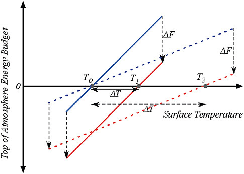
FIGURE 3.1 Determination of surface temperature response to a radiative forcing Δ F, in terms of the top-of-atmosphere energy budget. The top-of-atmosphere energy budget is the net of outgoing infrared radiation minus incoming solar radiation. The budget is zero when the system is in equilibrium. In these graphs, the budget is expressed schematically as a function of surface temperature. Equilibrium surface temperature is determined by the point where the line crosses the horizontal axis. If the system starts in equilibrium, but CO2 is increased so that the line is shifted downward by an amount Δ F (via reduction in outgoing infrared), then the intersection point shifts to warmer values by an amount Δ T. When the slope of the energy budget line is smaller, a given Δ F causes greater warming, as indicated by the pair of lines with reduced slope. This connects the slope of the energy budget line with climate sensitivity. The slope of the line is like the stiffness of a spring, and the radiative forcing Δ F is like the force with which one tugs on the spring. When the spring is not very stiff (e.g., a spring made of thin rubber bands) a given force will make the spring stretch to a great length—analogous to a large warming. If the spring is very stiff (e.g., a heavy steel garage door spring) the same force will cause hardly any stretching at all—analogous to low climate sensitivity. A spring with no stiffness at all would represent a very special case, demanding a specific physical explanation, just as would a case of zero slope of the energy budget line, which corresponds to infinite climate sensitivity.
to be closer to the Sun than Earth is, in order to make up for the lack of a greenhouse effect. The same greenhouse effect that keeps Earth from freezing over in its actual orbit reduces the temperature at which Earth radiates to space, reduces the slope characterizing the black-body feedback, and hence increases the sensitivity. Taking into account the greenhouse effect
TABLE 3.2 Key Physics and Processes Contributing to Climate Sensitivity (warming expected if carbon dioxide doubles from an unperturbed value of 278 ppmv to 556 ppmv)
|
Black-body radiation alone, ignoring the greenhouse effect of the unperturbed atmosphere |
0.7ºC |
|
Black-body radiation but also including the greenhouse effect in the unperturbed atmosphere |
0.9ºC |
|
As above, but also including well-documented feedbacks due to tropospheric water vapor changing at fixed relative humidity and changes in the lapse rate (vertical structure of the atmosphere), no clouds |
1.5ºC |
|
As above, also including clouds but keeping them fixed |
1.8ºC |
|
As above, including clouds and allowing the clouds to vary, along with other feedbacks such as snow and sea ice retreat, from IPCC AR4 suite of models |
Best estimate 3.2ºC Likely range 2.1-4.4ºC |
of the unperturbed (background) atmosphere gives Δ T2X of about 0.9ºC in the absence of clouds.1 But abundant evidence and basic physics shows that atmospheric water vapor must increase in a globally warmer world, and multiple lines of evidence confirm that both the atmosphere and general circulation models conform to a feedback that acts approximately as if the relative humidity is kept fixed (Held and Soden, 2000; Pierrehumbert et al., 2007; Dessler and Sherwood, 2009). When this result is used to incorporate the water vapor feedback into calculations of Earth’s infrared emission to space, and the lapse rate feedback is also taken into account, we find that Δ T2X increases to 1.5ºC. This figure is helpful for understanding the physics contributing to climate sensitivity, but it is incomplete because it is only for clear sky conditions. In the real atmosphere, clouds contribute to Earth’s background greenhouse effect, and their possible changes represent a key feedback.
The feedbacks that modify the basic black-body feedback are at the heart of predicting future climate. The combined water vapor and lapse rate feedback increases climate sensitivity by affecting the infrared emission side of the balance. Snow and sea-ice retreat work instead on the solar absorption side, but they also increase the sensitivity. Clouds work on both the infrared and solar side, and their net influence on sensitivity can go either way.
A quantitative treatment of cloud, snow, relative humidity, and sea-ice feedbacks requires the use of general circulation models. The estimates of equilibrium climate sensitivity in this report will be based on simulations employing mixed layer ocean models, which are thought to closely mimic
more complete simulations on longer time scales, once the ocean stops taking up heat.
For the general circulation models listed in Table 8.2 of IPCC, Working Group I, The Physical Science Basis (IPCC, 2007a), the equilibrium Δ T2x has a minimum of 2.1ºC, a maximum of 4.4ºC, and a median of 3.2ºC. Even the least sensitive model has a higher climate sensitivity than the idealized calculations yield for basic clear-sky water vapor and lapse-rate feedback. This is largely because the presence of clouds increases the basic black-body plus water vapor feedback sensitivity to about 1.8ºC even if clouds do not change as the climate warms. This form of cloud effect is not conventionally counted as a cloud feedback. It is more robust than feedbacks due to changing clouds, because it is based on cloud properties that can be verified against today’s climate. This value, too agrees well among models and is considered to be highly certain. Thus, the least sensitive IPCC models correspond very nearly to cloud properties remaining fixed while warming is amplified by water vapor feedbacks alone. The more sensitive models are more sensitive primarily by virtue of having positive cloud feedback. The spread in equilibrium climate sensitivity within the IPCC ensemble of models is primarily due to differences in cloud feedback, and in particular to the feedback of low clouds (Bony et al., 2006). Note that climate sensitivity could only be lower than about 1.8ºC if there are negative feedbacks very different from those of any of the models, such as changes in upper tropospheric or lower stratospheric water vapor, or changes in clouds that are opposite to those expected.
It has long been recognized that a symmetric distribution of the uncertainty in the strength of the feedbacks affecting climate sensitivity results in a skewed distribution in the climate sensitivity itself, with a high probability of large values (e.g., Schlesinger, 1986).2 Roe and Baker (2007) attempt to use this property to argue that it will be extremely difficult to eliminate the significant possibility of very high climate sensitivities. However, there is no a priori reason to expect the uncertainty in the strength of the feedback
|
2 |
This can be understood by noting that the climate sensitivity is proportional to 1/(1-f), where f is the strength of the feedbacks, and is positive if the feedbacks are positive. If one starts with the value f = 0.5, then increasing f by 0.25, say, increases the sensitivity by 100%, or a a factor of two. Decreasing f by the same amount decreases the sensitivity by only 67%. One can also use Figure 3.1 to understand this result pictorially. Climate sensitivity is proportional to the reciprocal of the slope shown in the figure, with the magnitude of the slope determined by the strength of the feedbacks. A symmetric distribution of slopes does not result in a symmetric distribution of climate sensitivity. A symmetric distribution might include zero slope with a finite probability, resulting in infinite climate sensitivity, which, of course, is ruled out by the observed stability of the climate system. |
to be symmetric, especially when one considers observational constraints, such as those that are provided by paleoclimates, that constrain the equilibrium climate response directly rather than by constraining the strengths of feedbacks. Hannart et al. (2009) have highlighted the implications of the arbitrary assumptions regarding uncertainty in Roe and Baker’s analysis. Chapter 6 contains a brief discussion of paleoclimatic constraints consistent with the range of equilibrium sensitivities in Table 3.1
Perturbed physics ensembles, notably Stainforth et al. (2005), do show that there are physical mechanisms that can operate in climate models, which yield climate sensitivity well above the top of the IPCC range employed in Table 3.1. Such ensembles do exhibit a distribution of climate sensitivity with a fat tail skewed toward high values, much as one would expect from assuming a symmetric and broad uncertainty distribution in the total feedback strength. In perturbed physics ensembles, it is typical to admit members to the ensemble only if they pass through a “keyhole” requiring that the basic climate of that member is realistic enough to serve as a basis for predicting the future. If the keyhole is made too wide, it can allow unrealistic behaviors to pass through. This is evidently the case for the many of the anomalously high climate sensitivity cases seen in Stainforth et al. (2005), which require a very unrealistic moistening of the upper troposphere and lower stratosphere (Sanderson et al., 2008; Joshi et al., 2010). It cannot unequivocally be ruled out that some unknown future climate state could trigger the onset of such behavior of water vapor, but there is no good basis at present for evaluating the prospects that this might happen. As another example, working with an alternative model, Yokohata et al. (2005) illustrate how simulation of the Pinatubo eruption provides evidence against a version of the model with equilibrium sensitivity as high as 6K.
Our choice to emphasize the CMIP3/AR4 model range is based on the judgment that these models have been analyzed most fully by the research community, thanks in large part to the open archive created by the World Climate Research Program’s Couple Model Intercomparison Program and the Department of Energy’s Program for Climate Model Diagnosis and Intercomparison (http://www-pcmdi.llnl.gov/). The description of this range of equilibrium sensitivity in the CMIP3 models as “likely” is consistent with the conclusions of the review of Knutti and Hegerl (2008), which attempts to take into account observational constraints as well as model results.
In interpreting future climate impacts based on Table 3.1 it is important to keep in mind that these do not necessarily represent worst possible cases, even if defensible physical mechanisms leading to higher climate sensitivity have not yet been identified. Our judgment is that the likelihood
of very high equilibrium climate sensitivities cannot be quantified at this time. We recognize the importance to policy makers of quantitative statements concerning high sensitivities but do not attempt to address this issue further in this report.
We consider it to be more difficult to provide useful estimates of uncertainty in equilibrium climate sensitivity than in the transient climate response (Section 3.3), due to the stronger observational constraints on the latter arising from observations on multidecadal-to-century time scales. In Table 3-1, we suggest values for the likely (66%) and very likely (90%) ranges for the transient climate response based on the discussion is Section 3.3
We are cognizant that current climate models have limitations, especially resulting from deficiencies in cloud simulations and in simulations of tropical convection. We do not try to delineate these deficiencies here or relate them to uncertainties in sensitivity. We rely on a general consistency between the range of sensitivities in the AR4 models and various observational constraints. The latter are discussed in Section 3.3 as they relate to the transient climate response and in Section 6.1 on longer time scales.
The equilibrium global mean temperature change results shown in Table 3.1 were computed by logarithmic extrapolation from the equilibrium climate sensitivity values reported for the 17 general circulation models in Table 8.2 of IPCC, Working Group I, The Physical Science Basis (IPCC, 2007a).3 Over the range of CO2 covered in the table, logarithmic extrapolation is equivalent to assuming temperature change to be linear in radiative forcing.
On time scales longer than a few years, the oceanic mixed layer and the atmosphere warm as a unit. However, heat loss out of the bottom of the mixed layer keeps the warming below the equilibrium value until the deep ocean has warmed up and equilibrated. It takes a great deal of energy to warm the deep ocean, and consequently it takes many centuries for the temperature to relax to the equilibrium warming. The idealized situation in which CO2 is held fixed for many centuries through carefully defined and ever decreasing emissions is unrealistic, and this might seem to make the equilibrium sensitivity a concept of mostly academic interest. Nonetheless, if used properly, the equilibrium climate sensitivity yields important informa-
tion about the long-term evolution of climate. As discussed in Chapter 2, if the emissions are reduced to zero after some fixed time, the CO2 peaks at the time of cessation of emissions, and very gradually relaxes back to smaller values over the subsequent millennia. Over the first few centuries, the warming in any given year will fall short of the equilibrium value expected from the CO2 concentration prevailing in that year, but during the long, slow decline of CO2, the temperature has time to catch up to the equilibrium curve. This form of approach to equilibrium is illustrated in the simulation shown in Figure 3.2. On time scales longer than about a thousand years, the equilibrium sensitivity applied to the instantaneous CO2 value provides a good estimate of the warming.
The approach to equilibrium takes long enough that slow feedback processes can intervene and alter the long-term climate evolution. This will be taken up in Chapter 6, where it will be shown that the persistent warming computed on the basis of equilibrium climate sensitivity provides a valuable guide as to whether the human imprint on climate is likely to be
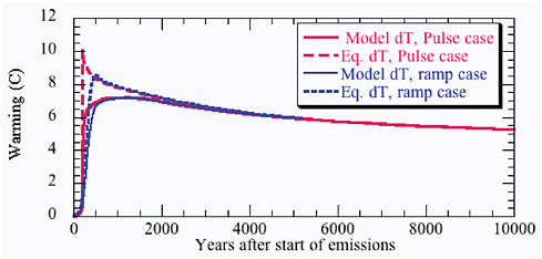
FIGURE 3.2 Comparison of equilibrium warming based on instantaneous CO2 values with actual modeled temperatures from Eby et al., 2009. The simulation shown is based on cumulative emission of 3840 Gt carbon in the form of CO2. Results are shown both for a pulse emission and for an exponentially increasing ramp lasting 350 years. “Instantaneous equilibrium warming” at any given moment in time is defined as the warming that would ultimately be reached in equilibrium if the CO2 prevailing at that moment were held fixed indefinitely. It provides an accurate estimate of the actual warming corresponding to the time varying CO2 when the CO2 concentrations are varying sufficiently slowly. In computing the instantaneous equilibrium warming, the climate sensitivity is held fixed at the value appropriate to the model used in the simulation. The equilibrium curves are proportional to the logarithm of the CO2 time series produced by the carbon cycle model used in this simulation. For this model Δ T2X is approximately 3.5 C.
of sufficient magnitude and duration to trigger significant effects from slow climate system feedbacks.
3.3
TRANSIENT CLIMATE RESPONSE AND SENSITIVITY
The climate system responds differently to perturbations in radiative forcing on different time scales. It is of special importance to carefully distinguish between the “equilibrium climate sensitivity” and the “transient climate response.” The concept of equilibrium climate sensitivity and its alternative definitions have been discussed in Section 3.2. The transient climate response is of special relevance for climate change over the 20th and 21st centuries.
The transient climate response, or TCR, is traditionally defined in a model using a particular experiment in which the atmospheric CO2 concentration is increased at the rate of 1% per year. The increase in global mean temperature in a 20-year period centered at the time of doubling (year 70) is defined as the TCR (Cubasch, 2001). The upper tens of meters of the ocean, the atmosphere, and the land surface are all strongly coupled to each other on time scales greater than a decade, and are expected to warm coherently with a well-defined spatial pattern during a period of increasing radiative forcing. (This pattern is discussed in Section 4.1.) On these time scales, the rate of change of the heat stored in oceanic surface layers, as well as the atmosphere and land surface, can be ignored to first approximation, and we can think of global mean temperature as determined by the energy balance between the radiative forcing F, the change in the radiative flux at the top of the atmosphere U, and the flux of energy D into the deeper layers of the ocean that are far from equilibrium: F = U + D.
On long enough times scales, as long as a millennium by some estimates (e.g., Stouffer, 2004), the heat flux into the deep ocean D tends to zero, and the climate response approaches its equilibrium value determined by the balance between F and U. On the shorter times scales at which the changes in the deep ocean are still small, the heat uptake grows in time roughly proportional to the global mean temperature perturbation, D = γT (Gregory and Mitchell, 1997; Raper et al., 2002; Dufresne and Bony, 2008), similar to the more familiar linear approximation to the radiative flux response, U = βT. The implication is that on these time scales we can use the simple approximation T = F/(β + γ).
This approximation is useful on a limited range of time scales—longer than a decade but shorter than the centuries required for the heat uptake by the oceans to begin to saturate (Gregory and Forster, 2008; Held et al.,
2010). It is also useful for the canonical 1% peryr experiment, so we can set TCR = F2X/(β + γ), where F2X equals the forcing due to doubling of CO2. We can then use the same proportionality constant, 1/(β + γ), to interpret 20th century warming and 21st century projections given only the evolution of the forcing F over time. As an example, Gregory and Forster (2008) show how the same proportionality constant between forcing and global mean temperature holds in a particular GCM for all of the 21st century forcing scenarios utilized by the AR4 and pictured in Figure 3.3 (IPCC, 2007c). The lack of separation of these different scenarios in the first half of the 21st century is not primarily due to some inertia in the physical climate system, but rather to the fact that the net radiative forcings in the various scenarios do not substantially diverge until the latter half of the century.
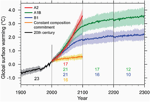
FIGURE 3.3 In stabilization scenarios, such as A1B (green) and B1 (blue) after 2100, or the “constant composition commitment” (yellow) in which the forcing is held fixed at the values in 2000, the warming grows slowly despite the constant forcing. Rescaling the TCR by the forcing will underestimate the surface warming in the stabilization period by an amount that grows with time, as the system slowly makes its transition to its equilibrium response. The average ratio of TCR to the equilibrium sensitivity in the models utilized by the AR4 (using values in Table 8.2 in Chaper 8 of the WG1 report) is 0.55. So the slow growth in the stabilization period, in which the forcing is somehow maintained at a constant level, continues for many centuries beyond that indicated in this figure, until the additional warming in these periods becomes comparable to that in the preceding periods of increasing forcing.
The ratio of TCR to the equilibrium response is smaller than one would expect from the linear analysis described above, using the mean value for these models of the heat uptake efficiency γ (Dufresne and Bony, 2008) and the radiative restoring β implied by the equilibrium climate sensitivity of these models. The explanation is that the strength of the restoring force provided by energy fluxes escaping to space, β, is found to decrease in climate models as the deep oceans equilibrate (Williams et al., 2008; Winton et al., 2010). In the CMIP3 archive the value of the radiative restoring relevant on the time scale of the 20th and 21st centuries is larger than the value relevant for the equilibrium response—by 30% on average, but with considerable model-to-model variations. This weakening of the radiative restoring once the deep oceans equilibrate is likely associated with changes in the horizontal structure of the warming. In the period of increasing forcing, the warming of the subpolar oceans is held back by strong coupling to the deep oceans. After stabilization, the deep oceans slowly warm and polar regions are thereby allowed to warm more rapidly, relative to the average warming of Earth’s surface. The radiative restoring is weaker for warming of the subpolar surface than for warming elsewhere because the coupling between the surface and tropospheric layers from which most of the radiation escaping to space is emitted is relatively weak in subpolar latitudes. The result is a reduction in the strength of the radiative restoring per degree warming of Earth’s surface as a whole.
The forcing due to well-mixed greenhouse gases (WMGGs) from the mid-19th century till 2010 is estimated to be 2.7 W/m2 by NOAA’s annual greenhouse gas index (http://www.esrl.noaa.gov/gmd/aggi/), which is about two-thirds of the forcing due to doubling of CO2 of about 3.7 W/m2. Therefore, one can estimate the warming due to the WMGGs since the mid-19th century, for a given value of TCR, as roughly two-thirds of TCR.
The distribution of TCR values generated by the CMIP3 models, as tabulated in Chapter 8 of the WG1/AR4 report (Randall et al., 2007), is displayed as a histogram in Figure 3.4. The mean, or median of this distribution, and the spread of values about this mean, are of interest in describing the values emerging from the best efforts of the major modeling groups around the world. The mean is between 1.8ºC and 1.9ºC and is somewhat larger than the median, which is close to 1.6ºC.
To explain the 20th century warming (0.7-0.8ºC) with WMGGs would require Earth to reside at the extreme low end of this distribution. As stated in the SPM of WG1/AR4, “it is likely that increases in greenhouse gases concentrations alone would have caused more warming than observed because volcanic and anthropogenic aerosols have offset some warming that would
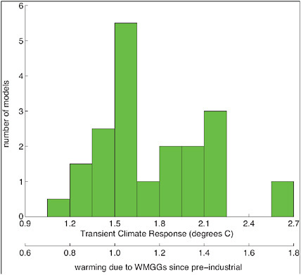
FIGURE 3.4 A histogram of TCR from a set of 19 models from 1% per year experiments described in Ch. 8 of WG1/AR4. The TCR values have also been converted into the warming since the mid-19th century due to well-mixed greenhouse gases by multiplying by 2/3.
otherwise have taken place” (IPCC, 2007c). In particular, a negative forcing of 0.8 W/m2 due to non-WMGG forcing, or a total forcing of 1.9 W/m2, would be consistent with the 20th century warming if TCR were roughly 1.5ºC—while a negative forcing of 1.2 W/m2, or total forcing of 1.5 W/m2, would be consistent with a TCR of about 1.9ºC. Total aerosol forcing of this magnitude is consistent, for example, with the estimate of Quaas et al. (2008), but the range of estimates is large.
Best estimates of TCR typically range from 1.5-2ºC. For example, Stott et al. (2006) use fingerprinting techniques to adjust the results from GCMs to improve fits to the spatial structure of observations and obtain a best estimate close to 2ºC. Knutti and Tomassini (2008) use a simple model to fit the 20th century temperature record and ocean heat uptake, using a Bayesian analysis to determine optimal parameters and uncertainties. Their best estimate for TCR is 1.5-1.6ºC, with a sharp cutoff at 1 and with a fairly long
tail on the high sensitivity end. The cutoff at 1 is common to most estimates, related to the fact that lower values of TCR requires positive forcing from unknown forcing agents or very large contributions to the century long trend from internal variability unlike any produced by current GCMs.
The temperature record over the past 30 years provides a potentially useful constraint on TCR (Gregory and Forster, 2008; Murphy et al., 2009). The anthropogenic aerosol forcing, although it has probably grown over much of the industrial era, was likely slowing if not fully leveling off over this period, leaving the well-mixed greenhouse gas forcing more dominant. Additionally, solar forcing, which is well constrained by satellite measurement of total solar irradiance, contributed very little to the trend over this period. Removing estimates of volcanic and ENSO signals from the global mean temperature record results in a fairly linear residual (e.g., Lean and Rind, 2009; Thompson et al., 2009). The residual yields a warming of about 0.48 K, or 0.16 K/decade, over the 30-year period. The WMGG forcing over this period is close to 1 W/m2. Rescaling implies a TCR of 1.8ºC, similar to the estimate of Gregory and Forster. Murphy et al. (2009), estimating TCR directly from TOA fluxes and ocean heat uptake over a similar time period, paint a picture consistent with relatively flat aerosol forcing in recent decades and a TCR of around 1.8.
The difficulty in using this relatively short period for estimating TCR is that internal climate variations are capable of modifying this trend substantially, so we cannot assume that the observed trend is entirely forced. Gregory and Forster (2008) estimate uncertainty by using the variability in 30-year trends of global mean temperature from a particular GCM. Their result is 1.3-2.3ºC as the 90% confidence interval around their best estimate of 1.8ºC. This is about the same range as in the CMIP3 models, but with a very different source of uncertainty. The Gregory and Forster estimate of uncertainty assumes that we have no information as to whether the contribution from internal variability was positive or negative during this period, although the CMIP3 range of values is due to uncertain physics in the models, especially cloud feedbacks.
There is a body of work on multi-decadal variability, especially in the North Atlantic, which suggests that internal variability has contributed positively to the temperature trends over the past 30 years. If correct, this would lower estimates of TCR that are based on comparison to temperature trends in recent decades. The North Atlantic is likely to be the source of much of the multi-decadal variability, and a variety of oceanographic and coupled model studies (Zhang, 2008; Knight, 2009; Latif et al., 2009; Polyakov et al., 2009) indicate that the North Atlantic has been in a warm phase over much
of this period. Polyakov et al. estimate that as much as 50% of the trend over this period in the North Atlantic is internal variability. The modeling work by Zhang and Knight also indicate that the influence of the Atlantic, despite its small size, can spread preferentially over Eurasia and contribute to global temperature signals. For example, the model analyzed by Knight generates a 0.1 K global mean warming for an increase of 1 Sverdrup (about 5% of the 20 Sverdrup mean value) in the Atlantic overturning.
Volcanic responses and the response to the 11-year solar cycle can also be used to constrain TCR, as can the autocorrelations of internal fluctuations (rather than watching the volcanic response decay in time to estimate the strength of restoring forces, one can watch internal fluctuations decay). Paeloclimatic evidence constrains equilibrium sensitivity, and with modeling guidance and heat uptake measurements constraining the ratio of TCR to the equilibrium response, one can also use these to constrain TCR. But there are also issues related to the decoupling of transient and equilibrium responses and to issues of “Earth system sensitivity”, that come into play when considering paleoclimatic constraints (see Chapter 6). We judge the constraints that directly involve fits to the temperature record over the past century and the last few decades to be the most useful in constraining TCR at this time.
The magnitude of many of the impacts discussed in this report scale with the value of TCR. We estimate TCR by starting with the distribution in the CMIP3 ensemble, but lowering the low end of the distribution slightly to take into account the possibility suggested by some recent studies of internal variability that a portion of the most recent Northern Hemisphere warming is internal. This results in a best estimate of 1.65ºC, likely lying in the range 1.3-2.2ºC (i.e., with 2/3 probability) and very likely lying in the range of 1.1-2.5ºC (i.e., with 90% probability). The estimate in the WG1/AR4 report is a very likely range of 1-3ºC. Our reduction of the upper limit to this range is consistent with our critique of very high equilibrium sensitivities in Section 3.2.
3.4
CUMULATIVE CARBON
Introduction: Why Use Cumulative Carbon Emissions?
The temperature response to anthropogenic carbon emissions is determined by: (1) the response of the carbon cycle to emissions; (2) the climate response to elevated CO2 concentrations; and (3) the feedback between climate change and the carbon cycle. There has been significant attention
in recent literature on how carbon sinks (and resultant airborne fraction) are affected by both elevated CO2 and climate changes (concentration-carbon and climate-carbon feedbacks; see Friedlingstein et al., 2006, Gregory et al., 2009, and Section 2.4). There is also a large body of literature aimed at estimating the temperature response to elevated CO2, typically defined as equilibrium climate sensitivity or transient climate response (Meehl et al., 2007; see also Sections 3.2 and 3.3). Each stage in the progression from carbon emissions to the resultant climate warming carries large uncertainty due to our incomplete understanding of the magnitude of both physical and biochemical feedbacks in the climate system.
Matthews et al. (2009) proposed a new metric of the temperature response to carbon emissions, the “carbon climate response,” which includes the net effects of both carbon cycle and physical climate feedbacks. The carbon-climate response is defined as the globally averaged temperature response to 1 trillion tons of carbon emissions (3.7 trillion tons of CO2), thus framing the climate response to emissions in the context of cumulative emissions of carbon dioxide over time. In effect, the carbon-climate reponse is a generalization of the concept of climate sensitivity as it pertains to carbon dioxide forcing. By including the carbon cycle response to emissions in addition to the temperature response to CO2 forcing, the carbon-climate response represents a metric that relates global mean temperature change directly to cumulative carbon emissions. This concept of measuring the climate response to cumulative emissions was also proposed concurrently by three other studies (Allen et al., 2009; Meinshausen et al., 2009; Zickfeld et al., 2009), all of which demonstrated a remarkably consistent temperature response to a given level of cumulative carbon emissions. Although CO2 radiative forcing decreases logarithmically with increasing CO2 concentrations, this is balanced by a near-exponential increase in the airborne fraction of emissions due to weakening carbon sinks at higher CO2 concentrations (Caldeira and Kasting, 1993). As a result, global mean temperature change is almost linearly related to cumulative carbon emission and is independent of the time during which the emissions occur (Matthews et al., 2009).
Estimates of the Temperature Response to Cumulative Emissions
Matthews et al. (2009) estimated the temperature response to cumulative carbon emissions as 1-2.1ºC per trillion tons of carbon (1000 GtC) emitted, based both on 21st century simulations by coupled climate-carbon cycle models and on historical observations of CO2-induced temperature change and anthropogenic CO2 emissions (Figure 3.5). This study produced a best
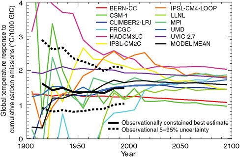
FIGURE 3.5 Temperature response to cumulative carbon emissions from coupled climate-carbon model simulations (thin colored lines) and historical observations of CO2-induced warming and anthropogenic CO2 emissions (thick black line solid and dotted lines). (Figure adapted from Figures 3 and 4 of Matthews et al., 2009).
estimate of 1.5ºC/1,000 GtC emitted based on observational constraints, and 1.6ºC/1,000 GtC based on the model average. Allen et al. (2009), using a simpler climate model but considering a larger range of climate sensitivity, found a most likely peak temperature response of 2ºC/1,000 GtC, with a 5-95% confidence range of 1.3-3.9ºC/1,000 GtC. Allen et al. also provided an estimate for the instantaneous temperature response to cumulative emissions (corresponding to the definition of the carbon-climate response from Matthews et al.) of 1.4-2.5ºC/1,000 GtC. Both Matthews et al. (2009) and Allen et al. (2009) concluded that the temperature response to cumulative emissions is remarkably constant over time and over a wide range of CO2 emissions scenarios. Based on this, they provided best estimates of the allowable emissions for 2ºC global temperature increase of 1,000 GtC (Allen et al., 2009) and 1,300 GtC (Matthews et al., 2009).
Zickfeld et al. (2009) also presented an estimate of the cumulative emissions required to meet a 2ºC temperature target. The authors considered both climate sensitivity uncertainty and the uncertainty in climate-carbon feed-
backs, and thus were able to generate a probabilistic estimate of the emissions associated with various temperature targets. To restrict the probability of exceeding 2ºC to 33%, Zickfeld et al. concluded that emissions from 2001 to 2500 must be kept to a median estimate of 590 GtC, with a range of 200 to 950 GtC owing to different estimates of climate sensitivity uncertainty, as well as uncertainty in climate-carbon feedbacks. For an exceedence probability of 50%, the median estimate from this study was approximately 840 GtC (range: 500 to 1,210). Including also historical CO2 emissions up to 2000 (~460 GtC; Houghton, 2008; Boden et al., 2009), this best estimate for 2ºC from Zickfeld et al. corresponds to emissions of approximately 1,050 GtC (1,300 GtC) for an exceedence probability of 33% (50%). Meinshausen et al. (2009) also presented an estimate of the cumulative carbon emissions required to meet a 2ºC temperature target. This study used a simpler model and a narrower time window (2000-2050) but considered also the effect of non-CO2 greenhouse gases and aerosols; Meinshausen et al. estimated that cumulative emission from 2000-2050 must be restricted to 390 GtC to avoid 2ºC warming with 50% likelihood.
“Stabilization” Framework Based on Cumulative Carbon
The cumulative carbon framework is well suited to relating instantaneous global temperature change to a given level of cumulative carbon emitted. Based on the above studies, we select 1.75ºC global temperature change per 1,000 GtC emitted to be a representative best estimate for the climate response to cumulative carbon emissions. There is large uncertainty, however, in this estimate of the temperature response to carbon emissions owing both to uncertain carbon cycle response to elevated CO2 and climate changes (Section 2.4) as well as to uncertainty in the physical climate system response to CO2 forcing (Sections 3.2 and 3.3). We use here a very likely uncertainty range on this central estimate of 1 to 2.5ºC per 1,000 GtC emitted, based on the lower and upper 5-95% confidence limits given in Matthews et al. (2009) and Allen et al. (2009).
This estimate of the temperature response to cumulative emissions corresponds to approximately 1,150 GtC (4200 billion tons of CO2) in allowable emissions consistent with 2ºC temperature change (Figure 3.6). It is critical to recognize, however, that the uncertainty range on this number is very large, with a possible lower limit of 500 GtC (1,800 Gt CO2) inferred from Allen et al. (2009) and a possible upper limit of 1,900 GtC (7000 Gt CO2) from Matthews et al. (2009); this range of CO2 emissions (500-1,900 GtC) can be considered to be a very likely range for emissions consistent with 2ºC global warming. We can narrow this range somewhat and apply
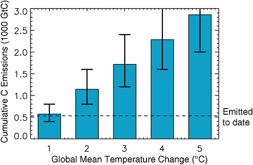
FIGURE 3.6 Cumulative carbon emissions consistent with global mean temperature changes of 1 to 5ºC. Best estimates are based on 1.75ºC per 1,000 GtC emitted, taken as a representative best estimate from Matthews et al. (2009) and Allen et al. (2009). Likely uncertainty ranges of 70-140% of the best estimate are based on Zickfeld et al. (2009) and Matthews et al. (2009). The dashed line shows cumulative emission to the year 2009 (530 GtC).
it to other warming levels based on a combination of the results of Zickfeld et al. (2009) and Matthews et al. (2009). Matthews et al. (2009) presented a 5-95% uncertainty range of 1,000 to 1,900 GtC on emissions for 2ºC, based on a central estimate of 1400 GtC; this corresponds to a uncertainty range of approximately 70-140% of the central estimate. Zickfeld et al. (2009) also provided an uncertainty range for the cumulative emissions associated with 2, 3, and 4ºC global mean temperature change, and found that the relative uncertainty scaled approximately with the median value. Based on this, we use the relative uncertainty range from Matthews et al. (2009) and apply this to our central estimate of emissions consistent with each temperature target. For 2 degrees, this represents a best estimate of 1,150 GtC, with an uncertainty range of 800 to 1,600 GtC (Figure 3.6), which we adopt here as the likely range of emissions for 2ºC global warming.
While global mean temperature change is well constrained by cumulative emissions, this cumulative carbon framework is less consistent with the more widely used framework of CO2 concentration stabilization. A given
level of cumulative CO2 emissions do not result in stable CO2 concentrations, but rather in CO2 concentrations that peak at some value and then decrease slowly when emissions fall below the level of persistent natural carbon sinks (see Figure 3.7). For rates of emission reduction of the order of 1-4% per year, and even if CO2 emissions become close to zero, the decrease in atmospheric concentrations may, however, occur very slowly over
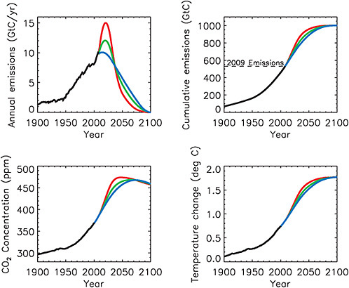
FIGURE 3.7 Illustrative emissions scenarios with cumulative emissions from 1750 to 2100 totaling 1,000 GtC (3,700 GtC). For all scenarios, the year-2100 temperature change and CO2 concentration do not depend on the shape of the emissions scenario, but rather on the total cumulative emitted. These scenarios were constructed such that total cumulative carbon emissions were the same for each scenario, the rate of emissions decline varied from 1.5 to 4. 5% per year relative to the peak emissions, and emissions were constrained to reach zero at the year 2100. CO2 concentrations and temperature changes shown here were simulated by the UVic ESCM. Source: Weaver et al. (2001) and Eby et al. (2009).
centuries (see Section 2.2). In a framework of cumulative carbon emissions, CO2 concentrations do not necessarily “stabilize” but rather change over time in response to a given CO2 emissions scenarios; in this case, it is the total cumulative carbon emitted over time, rather than the atmospheric CO2 concentration itself, that indicates the level of expected climate warming.
The clear advantage of the cumulative carbon framework is that a given level of cumulative emissions corresponds to a unique temperature change, which remains approximately constant for several centuries after the point of zero emissions (Matthews et al., 2008; Solomon et al., 2009). As can be seen in Figure 3.7, for this particular model, cumulative emissions of 1,000 GtC from 1750 to 2100 result in a year-2100 global temperature change of 1.8ºC over pre-industrial temperatures, which corresponds to a year-2100 CO2 concentration of 460 ppm; both the year-2100 temperature change and the year-2100 CO2 concentration are independent of the shape of the CO2 emissions scenario and depend only on the total cumulative carbon emitted. By contrast, the rate of temperature change, as well as the peak CO2 concentration in these simulations, varied as a results of differences in the rates of increase and decline of emissions in each scenario.
Figure 3.8 illustrates how the concept of CO2 stabilization can be reconciled with the cumulative emissions framework. This figure shows idealized CO2 concentration scenarios that reach between 350 and 1,000 ppm at the year 2100, along with the cumulative carbon emissions and temperature changes associated with each scenario.4 From this analysis, restricting global temperature change to 2ºC requires best-guess cumulative emissions of 1,150 billion tons of carbon between the years 1800 and 2100; this corresponds to a “stabilization” CO2 concentration of between 450 and 550 ppm at the year 2100, with the caveats that CO2 concentrations changes and warming after the year 2100 would depend on the level of additional post-2100 emissions. In general, at a given time (e.g., the year 2100) both the atmospheric CO2 concentration and the associated temperature change can be inferred from cumulative carbon emissions to date. If carbon emissions were subsequently eliminated, atmospheric concentrations would slowly decrease over time, whereas temperature would remain elevated for several
|
4 |
The temperature responses to cumulative emissions shown in Figure 3.8 include both the carbon cycle and climate sensitivity to emissions, but do not correspond directly to either the transient climate response or the equilibrium climate sensitivity associated with a given CO2 concentration. In general, for higher emissions scenarios where forcing is still increasing rapidly at 2100, this temperature change will more closely reflect the transient climate response. For lower emissions scenarios with stable or declining forcing during the latter half of the 21st century, the temperature change at 2100 will more closely reflect the equilibrium climate sensitivity. |
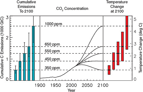
FIGURE 3.8 Idealized CO2 concentration scenarios reaching between 350 and 1,000 ppm at the year 2100. At the year 2100, the atmospheric CO2 concentration and global mean temperature change is dependent on cumulative carbon emissions to date, with variation in the rate of emissions over time affecting only the rate of increase of forcing and consequent rate of temperature change. Stabilization of CO2 concentrations after the year 2100 would require continued low-level CO2 emissions (leading to increasing cumulative carbon emitted), whereas zero emission after 2100 would result in slowly declining CO2 concentrations and approximately stable global temperature. Cumulative emissions for each scenario shown here are based on simulations with the UVic ESCM, with uncertainty ranges of 70-140% of the central value based on Matthews et al. (2009) and Zickfeld et al. (2009). Temperature changes are calculated using 1.75ºC per 1,000 GtC emitted, with a 1-2.5ºC/1,000 GtC uncertainty range based on Matthews et al. (2009) and Allen et al. (2009). These uncertainty ranges reflect both uncertainty in the response of carbon sinks to elevated CO2 and climate changes, as well as uncertainty in the physical climate system response to change in CO2 forcing.
centuries. Similarly, should emissions continue at a low level (resulting in increasing cumulative carbon emissions), atmospheric concentrations may remain stable, but global mean temperature would continue to increase over time. Atmospheric CO2 stabilization is consistent with a small amount of continued CO2 emissions at a rate equal to the level of persistent natural carbon sinks, whereas atmospheric temperature stabilization is only consistent with near-zero CO2 emissions (Matthews and Caldeira, 2008; Solomon et al., 2009).


