
9
DOMAIN STRETCHING
I. We are starting to close in on the Riemann Hypothesis. Let me state it again, just as a refresher.
The Riemann Hypothesis
All non-trivial zeros of the zeta function have real part one-half.
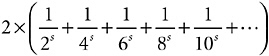
Well, we’ve got a handle on the zeta function. If s is some number bigger than 1, the zeta function is as shown in Expression 9-1.
Expression 9-1
or, to be somewhat more sophisticated about it
where the terms of the infinite sum run through all the positive whole numbers. I have showed how, by applying a process very much like the sieve of Eratosthenes to this sum, it is equivalent to
that is,
where the terms of the infinite product run through all the primes.
And so
which I have called the Golden Key.
So far, so good, but what is this about non-trivial zeros? What is a zero of a function? What are the zeros of the zeta function? And when are they non-trivial? Onward and upward.
II. Forget about the zeta function for a moment. Here is a completely different infinite sum.
S(x) = 1 + x + x2 + x3 + x4 + x5 + x6 + …
Does this ever converge? Sure. If x is ![]() , the sum is just Expression 1-1 in Chapter 1.iv, because
, the sum is just Expression 1-1 in Chapter 1.iv, because ![]() ,
, ![]() , etc. Therefore,
, etc. Therefore, ![]() , because that’s what that sum converged to. What’s more, if you think about the rule of signs,
, because that’s what that sum converged to. What’s more, if you think about the rule of signs, ![]() ,
, ![]() , etc. Therefore,
, etc. Therefore, ![]() , from Expression 1-2 in Chapter 1.v. Similarly, Expression 1-3 means that
, from Expression 1-2 in Chapter 1.v. Similarly, Expression 1-3 means that ![]() , while Expression 1-4 gives
, while Expression 1-4 gives
![]() . Another easy value for this function is S(0) = 1, since zero squared, zero cubed, and so on are all zero, and only the initial 1 is left standing.
. Another easy value for this function is S(0) = 1, since zero squared, zero cubed, and so on are all zero, and only the initial 1 is left standing.
If x is 1, however, S(1) is 1 + 1 + 1 + 1 + …, which diverges. If x is 2, the divergence is even more obvious, 1 + 2 + 4 + 8 + 16 + …. When x is –1 a weird thing happens. By the rule of signs, the sum becomes 1 – 1 + 1 – 1 + 1 – 1 + …. This adds up to zero if you take an even number of terms, to one if you take an odd number. This is definitely not going off to infinity, but it isn’t converging, either. Mathematicians consider it a form of divergence. For –2 things are even worse. The sum is 1 – 2 + 4 – 8 + 16 – …, which seems to go off to infinity in two different directions at once. Again, you definitely can’t call this convergence, and if you call it divergence, nobody will argue with you.
In short, S(x) has values only when x is between –1 and 1, exclusive. Elsewhere it has no values. Table 9-1 shows values of S(x) for arguments x between –1 and 1.
TABLE 9-1 Values of S(x) = 1 + x + x2 + x3 + …
|
x |
S(x) |
|
–1 or below |
(No values) |
|
–0.5 |
0.6666… |
|
–0.3333… |
0.75 |
|
0 |
1 |
|
0.3333… |
1.5 |
|
0.5 |
2 |
|
1 or above |
(No values) |
That’s all you can get from the infinite sum. If you make a graph, it looks like Figure 9-1, with no values at all for the function west of –1 or east of 1. If you remember the term of art, the domain of this function is from –1 to 1, exclusive.

FIGURE 9-1 The function S(x) = 1 + x + x2 + x3 + …
III. But look, I can rewrite that sum
S(x) = 1 + x + x2 + x3 + x4 + x5 + …
like this
S(x) = 1 + x(1+ x + x2 + x3 + x4 + …)
Now, that series in the parenthesis is just S(x). Every term that is in the one is also in the other. That means they are the same.
In other words, S(x) = 1 + xS(x). Bringing the rightmost term over to the left of the equals sign, S(x) – xS(x) = 1, which is to say (1 – x) S(x) = 1. Therefore, S(x) = 1/(1–x). Can it be that behind that infinite sum is the perfectly simple function 1 / (1 – x)? Can it be that Expression 9-2 is true?
Expression 9-2
It certainly can. If ![]() , for example, then 1 / (1 – x) is
, for example, then 1 / (1 – x) is ![]() , which is 2. If x = 0, 1 / (1 – x) is 1 / (1 – 0), which is 1. If
, which is 2. If x = 0, 1 / (1 – x) is 1 / (1 – 0), which is 1. If ![]() , 1 / (1 – x) is
, 1 / (1 – x) is ![]() , which is
, which is ![]() , which is
, which is ![]() . If
. If ![]() , 1/(1–x) is
, 1/(1–x) is ![]() , which is
, which is ![]() , which is
, which is ![]() . If
. If ![]() , 1 / (1 – x) is
, 1 / (1 – x) is ![]() , which is
, which is ![]() , which is
, which is ![]() . It all checks out. For all the arguments
. It all checks out. For all the arguments ![]() ,
, ![]() , 0,
, 0, ![]() ,
, ![]() , for which we know a function value, the value is the same for the infinite series S(x) as it is for the function 1 / (1 – x). Looks like they are actually the same thing.
, for which we know a function value, the value is the same for the infinite series S(x) as it is for the function 1 / (1 – x). Looks like they are actually the same thing.
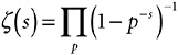
But they are not the same thing, because they have different domains, as Figures 9-1 and 9-2 illustrate. S(x) only has values between –1 and 1, exclusive. By contrast, 1 / (1 – x) has values everywhere, except at x = 1. If x = 2, it has the value 1 / (1 – 2), which is –1. If x = 10, it has the value 1 / (1 – 10), which is ![]() . If x =–2, it has the value 1 / (1 – (–2)), which is
. If x =–2, it has the value 1 / (1 – (–2)), which is ![]() . I can draw a graph of 1 / (1 – x). You see that it is the same as the previous graph between –1 and 1, but now it has values west of 1 and east of (and including) –1, too.
. I can draw a graph of 1 / (1 – x). You see that it is the same as the previous graph between –1 and 1, but now it has values west of 1 and east of (and including) –1, too.
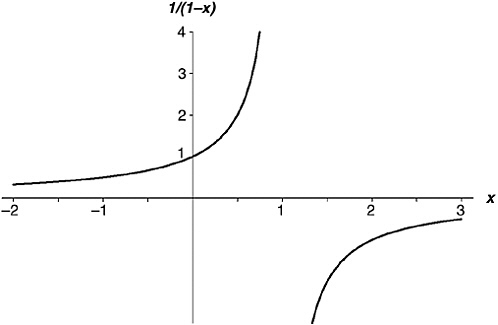
FIGURE 9-2 The function 1/(1 – x).
The moral of the story is that an infinite series might define only part of a function; or, to put it in proper mathematical terms, an infinite series may define a function over only part of its domain. The rest of the function might be lurking away somewhere, waiting to be discovered by some trick like the one I did with S(x).
IV. That raises the obvious question: is this the case with the zeta function? Does the infinite sum I’ve been using for the zeta function—Expression 9-1—describe only part of it? With more yet to be discovered? Is it possible that the domain of the zeta function
is bigger than just “all numbers greater than 1”?
Of course it is. Why would I be going to all this trouble otherwise? Yes, the zeta function has values for arguments less than 1. In fact, like 1 / (1 – x), it has a value at every number with the single exception of x = 1.
At this point, I’d like to draw you a graph of the zeta function showing all its features across a good range of values. Unfortunately, I can’t. As I mentioned before, there is no really good and reliable way to show a function in all its glory, except in the case of the simplest functions. To get intimate with a function takes time, patience, and careful study. I can graph the zeta function piecemeal, though. Figures 9-3 through 9-10 show values of ζ (s) for some arguments to the left of s = 1, though I have had to draw each to a different scale. You can tell where you are by the argument (horizontal) and value (vertical) numbers printed on the axes. In the scale marks, “m” means “million,” “tr” means “trillion,” “mtr” means “million trillion,” and “btr” means “billion trillion.”
In short, when s is just less than 1 (Figure 9-3), the function value is very large but negative—as if, when you cross the line s = 1 heading west, the value suddenly flips from infinity to minus infinity. If you
continue traveling west along Figure 9-3—that is, bringing s closer and closer to zero—the rate of climb slows down dramatically. When x is zero, ζ (s) is  . At s =–2 the curve crosses the s-axis—that is, ζ (s) is zero.
It then (we are still headed west, and now in Figure 9-4) climbs up to a modest height (actually 0.009159890…) before turning down and crossing the axis again at s =–4. The graph drops down to a shallow trough (–0.003986441…) before rising again to cross the axis at s =–6. Another low peak (0.004194), a drop to cross the axis at s = –8, a slightly deeper trough (–0.007850880…), across the axis at –10, now a really noticeable peak (0.022730748…), across the axis at s = –12, a deep trough (–0.093717308…), across the axis at s = –14, and so on.
The zeta function is zero at every negative even number, and the successive peaks and troughs now (Figures 9-5 to 9-10) get rapidly more and more dramatic as you head west. The last trough I show, which occurs at s = –49.587622654…, has a depth of about 305,507,128,402,512,980,000,000. You see the difficulty of graphing the zeta function all in one piece.
FIGURES 9-3 through 9-10 Graphs of ζ (s) when s is less than 1.
V. But how do I get these values for ζ (s) when s is less than 1? I’ve already shown that the infinite series in Expression 9-1 doesn’t work. What does work? If, to save my life, I had to calculate the value of ζ (–7.5), how would I set about it?
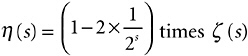
This I can’t fully explain, because it needs way too much calculus. I can give the general idea, though. First, let me define a new function, using an infinite series slightly different from the one in Expression 9-1. This is the η function; “η” is “eta,” the seventh letter of the Greek alphabet, and I define the eta function as
In a rough sort of way, you can see that this has a better prospect of converging than Expression 9-1. Instead of relentlessly adding numbers, we are alternately adding, then subtracting, so each number will to some extent cancel out the effect of the previous number. So it happens. Mathematicians can prove, in fact—though I’m not going to prove it here—that this new infinite series converges whenever s is greater than zero. This is a big improvement on Expression 9-1, which converges only for s greater than 1.
What use is that for telling us anything about the zeta function? Well, first note the elementary fact of algebra that A – B + C – D + E – F + G – H + … is equal to (A + B + C + D + E + F + G + H + …) minus 2 × (B + D + F + H + …).
So I can rewrite η (s) as

minus
The first parenthesis is of course just ζ (s). The second parenthesis can be simplified by Power Rule 7, (ab)n = anbn. So every one of those
even numbers can be broken up like this: ![]() , and I can take out
, and I can take out ![]() as a factor of the whole parenthesis. Leaving what inside the parenthesis? Leaving ζ (s)! In a nutshell
as a factor of the whole parenthesis. Leaving what inside the parenthesis? Leaving ζ (s)! In a nutshell
or, writing it the other way round and doing a last bit of tidying
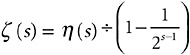
Now, this means that if I can figure out a value for η (s), then I can easily figure out a value for ζ (s). And since I can figure out values for η (s) between 0 and 1, I can get a value for ζ (s) in that range, too, in spite of the fact that the “official” series for ζ (s) (Expression 9-1) doesn’t converge there.
Suppose s is ![]() , for example. If I add up 100 terms of
, for example. If I add up 100 terms of ![]() I get 0.555023639…; if I add up 10,000 I get 0.599898768…. In fact,
I get 0.555023639…; if I add up 10,000 I get 0.599898768…. In fact, ![]() has the value 0.604898643421630370…. (There are shortcuts for doing this without adding up zillions of terms.) Armed with this, I can calculate a value for
has the value 0.604898643421630370…. (There are shortcuts for doing this without adding up zillions of terms.) Armed with this, I can calculate a value for ![]() ; it comes out to –1.460354508…, which looks pretty much right, based on the first one in that last batch of graphs.
; it comes out to –1.460354508…, which looks pretty much right, based on the first one in that last batch of graphs.
But hold on there a minute. How can I juggle these two infinite series at the argument ![]() , where one of the series converges and one doesn’t? Well, strictly speaking, I can’t, and I have been playing a bit fast and loose with the underlying math here. I got the right answer, though, and could repeat the trick for any number between zero and 1 (exclusive), and get a correct value for ζ (s).
, where one of the series converges and one doesn’t? Well, strictly speaking, I can’t, and I have been playing a bit fast and loose with the underlying math here. I got the right answer, though, and could repeat the trick for any number between zero and 1 (exclusive), and get a correct value for ζ (s).
VI. Except for the single argument s = 1, where ζ (s) has no value, I can now provide a value for the zeta function at every number s greater than zero. How about arguments equal to or less than zero? Here things get really tough. One of the results in Riemann’s 1859 paper proves a formula first suggested by Euler in 1749, giving
ζ (1 – s) in terms of ζ (s). So if you want to know the value of, say, ζ (–15), you can just calculate ζ (16) and feed it into the formula. It’s a heck of a formula, though, and I give it here just for the sake of completeness.48

Here π , in both occurrences, is the magic number 3.14159265…, “sin” is the good old trigonometric sine function (with the argument in radians), and ! is the factorial function I mentioned in Chapter 8.iii. In high school math, you meet the factorial function only in relation to positive whole numbers: 2! = 1 × 2, 3! = 1 × 2 × 3, 4! = 1 × 2 × 3 × 4, and so on. In advanced math, though, there is a way to define the factorial function for all numbers except the negative integers, by a domain-stretching exercise not unlike the one I just did. For example, ![]() turns out to be 0.8862269254…(half the square root of π , in fact),
turns out to be 0.8862269254…(half the square root of π , in fact), ![]() , etc. The negative integers create problems in the formula, but they are not major problems, and I shall say nothing about them here. Figure 9-11 shows the full factorial function, for arguments from –4 to 4.
, etc. The negative integers create problems in the formula, but they are not major problems, and I shall say nothing about them here. Figure 9-11 shows the full factorial function, for arguments from –4 to 4.
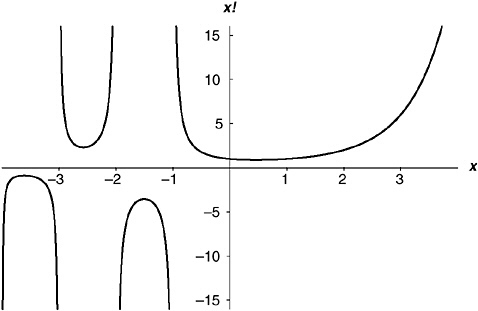
FIGURE 9-11 The full factorial function x!
If you find that a little over the top, just take it on faith that there is a way to get a value of ζ (s) for any number s, with the single exception of s = 1. Even if that last formula bounces right off your eye, at least notice this: it gives ζ (1 – s) in terms of ζ (s). That means that if you know ζ (16) you can calculate ζ (–15); if you know ζ (4) you can calculate ζ (–3); if you know ζ (1.2) you can calculate ζ (–0.2); if you know ζ (0.6) you can calculate ζ (0.4); if you know ζ (0.50001) you can calculate ζ (0.49999); and so on. The point I’m getting at is that the argument “one-half ” has a special status in this relationship between ζ (1 – s) and ζ (s), because if ![]() , then 1 – s = s. Obviously—obviously, I mean, from glancing at Figure 5-4 and Figures 9-3 through 9-10—the zeta function is not symmetrical about the argument
, then 1 – s = s. Obviously—obviously, I mean, from glancing at Figure 5-4 and Figures 9-3 through 9-10—the zeta function is not symmetrical about the argument ![]() ; but the vaues for arguments to the left of
; but the vaues for arguments to the left of ![]() are bound up with their mirror images on the right in an intimate, though complicated, way.
are bound up with their mirror images on the right in an intimate, though complicated, way.
Glancing back at that last bunch of graphs, you notice something else: ζ (s) is zero whenever s is a negative even number. Now, if a certain argument gives the function a value of zero, that argument is called “a zero of ” the function. So the following statement is true.
–2, –4, –6, … and all other negative even whole numbers are zeros of the zeta function.
And if you look back at the statement of the Riemann hypothesis, you see that it concerns “all non-trivial zeros of the zeta function.” Are we getting close? Alas, no, the negative even integers are indeed zeros of the zeta function; but they are all, every one of them, trivial zeros. For non-trivial zeros, we have to dive deeper yet.
VII. As an afterthought to this chapter, I am going to give my calculus a very brief workout, applying two of the results I stated in Chapter 7 to Expression 9-2. Here is that expression again, true for any number x between –1 and 1, exclusive.
Expression 9-2, again
All I intend to do is integrate both sides of the equals sign. Since the integral of 1 / x is log x, I hope it won’t be too much of a stretch to believe—I shall not pause to prove it—that the integral of 1 / (1 – x) is –log(1 – x). The right-hand side is even easier. I can just integrate term by term, using the rules for integrating powers that I gave in Table 7-2. Here is the result (which was first obtained by Sir Isaac Newton).
It will be a little handier, as you can see in Expression 9-3, if I multiply both sides by –1.
Expression 9-3
Oddly, though it makes little difference to the way I shall apply it, Expression 9-3 is true when x =–1, even though the expression I started with, Expression 9-2, isn’t. When x =–1, in fact, Expression 9-3 gives the result shown in Expression 9-4.
Expression 9-4
Note the similarity to the harmonic series. Harmonic series … prime numbers … zeta …. This whole field is dominated by the log function.
The right-hand side of Expression 9-4 is slightly peculiar, though this is not obvious to the naked eye. It is, in fact, a textbook example of the trickiness of infinite series. It converges to log 2, which is
0.6931471805599453…, but only if you add up the terms in this order. If you add them up in a different order, the series might converge to something different; or it might not converge at all!49
Consider this rearrangement, for example, ![]() Just putting in some parentheses, it is equal to
Just putting in some parentheses, it is equal to ![]() If you now resolve the parentheses, this is
If you now resolve the parentheses, this is ![]() , which is to say
, which is to say ![]() . The series thus rearranged adds up to one-half of the un-rearranged series!
. The series thus rearranged adds up to one-half of the un-rearranged series!
The series in Expression 9-4 is not the only one with this rather alarming property. Convergent series fall into two categories: those that have this property, and those that don’t. Series like this one, whose limit depends on the order in which they are summed, are called “conditionally convergent.” Better-behaved series, those that converge to the same limit no matter how they are rearranged, are called “absolutely convergent.” Most of the important series in analysis are absolutely convergent. There is another series that is of vital interest to us, though, that is only conditionally convergent, like the one in Expression 9-4. We shall meet that series in Chapter 21.


