Prime Obsession: Bernhard Riemann and the Greatest Unsolved Problem in Mathematics (2003)

I. Now I am going to try to make a run right for the heart of Riemann’s 1859 paper. This involves taking in some of Riemann’s math, which is very advanced. I shall skip nimbly over the really difficult parts, presenting them as faits accomplis, and just try to give the logical steps in Riemann’s argument by saying things like, “Mathematicians have a way to get from here to here,” without explaining what that way is, or why it works.

My hope is that you will end up with at least an outline of the main logical steps Riemann followed. I can’t do even that much, though, without a very small amount of calculus, the essential points of which I have already laid out in Chapter 7.vi-vii. You might find the following few sections challenging. The reward will be a result of great beauty and power, from which flows everything—the Hypothesis, its importance, and its relevance to the distribution of prime numbers.

II. To begin, I’m going to contradict something I said way back in Chapter 3.iv. Well, sort of contradict it. I said there wasn’t much point trying to draw a graph of the Prime Counting Function π (N). At that point in the book, there wasn’t. Well, now there is.

However, I am first going to make some slight adjustments. Instead of writing π (N), which, to the mathematical eye, translates as “the number of primes up to and including the natural number N,” I’m going to write π (x), which should be taken to mean “the number of primes up to and including the real number x.” This is not a big deal. Obviously the number of primes up to 37.51904283 inclusive is just the number of primes up to 37 inclusive, which is twelve: 2, 3, 5, 7, 11, 13, 17, 19, 23, 29, 31, 37. But we are heading for some calculus, so we want to be in the realm of numbers at large, not just whole numbers.

And one more adjustment. As I advance the argument x smoothly through a range of values, π (x) is going to make sudden jumps. Suppose x moves smoothly from 10 to 12, for example. The number of primes less than 10 is 4 (2, 3, 5, and 7), so the function value is 4 when x = 10, and also of course when x = 10.1, 10.2, 10.3, and so on. At argument 11, however, it will suddenly jump to 5; and for 11.1, 11.2, 11.3, … the value will hold at a steady 5. This is what mathematicians call a “step function.” And here is an adjustment rather commonly made with step functions. At precisely the point where π (x) jumps, I am going to give it a value half-way up the jump. So at argument 10.9, or 10.99, or 10.999999, the function value is 4; at argument 11.1, or 11.01, or 11.000001, the function value is 5; but at argument 11 it is 4.5. I am sorry if this seems a little wacky, but it is essential for what follows. If I do this, then all the arguments in this chapter and Chapter 21 work; if I don’t, they don’t.

Now I can show a graph of π (x) (see Figure 19-1). Step functions are a little hard to get used to at first, but from a mathematical point of view they are perfectly sound. The domain here is all non-negative numbers. In that domain, every argument has a single

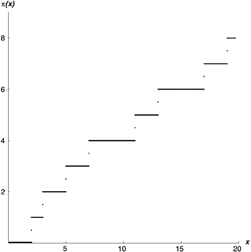
FIGURE 19-1 The prime counting function.

unique value. Give me an argument, I’ll give you a value. Math has much stranger functions than this.

III. Now I am going to introduce another function, also a step function, just a little bit odder than π (x). Riemann, in his 1859 paper, calls it the “f ” function, but I’m going to follow Harold Edwards and refer to it as the “J” function. Since Riemann’s time, mathematicians have got into the habit of using “f ” to represent a generic function, “Let f be any function…,” so it’s a bit difficult for them to see f as referring to a particular function.

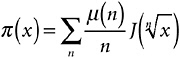
OK, here goes with the definition of the J function. For any non-negative number x, the J function has the value shown in Expression 19-1.

Expression 19-1

The symbol “π ” here is the Prime Counting Function as defined up above, for any real number x.

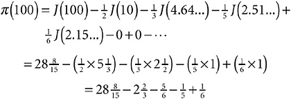
Notice that this is not an infinite sum. To see why not, consider some definite number x, say, x = 100. The square root of 100 is 10; the cube root is 4.641588…; the fourth root is 3.162277…; the fifth root is 2.511886…; the sixth root is 2.154434…; the seventh root is 1.930697…; the eighth root is 1.778279…; the ninth root is 1.668100…, and the tenth root is 1.584893…. I could, of course, go on working out the eleventh, twelfth, thirteenth roots, and so on for as far as you please. I don’t need to, though, because the prime counting function has a very nice property; if x is less than 2, π (x) is zero, because there aren’t any primes less than 2! In fact I could have stopped calculating roots of 100 after the seventh. What I have in this case is

which, if you count up primes, means

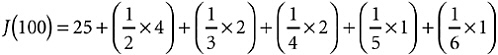
and that works out to , or 28.53333…. If you keep taking roots of any number, sooner or later the root drops below 2, and all the terms in the J function from there on are zero. So for any argument x, the value of J(x) can be worked out from a finite sum—a great improvement over some of the functions we’ve been dealing with!

This J function is, as I said, a step function. Figure 19-2 shows what it looks like for arguments up to 10. You can see that the J function jumps suddenly from one value to another, holds the new value for a while, then makes another jump. What are these jumps? What’s the pattern?

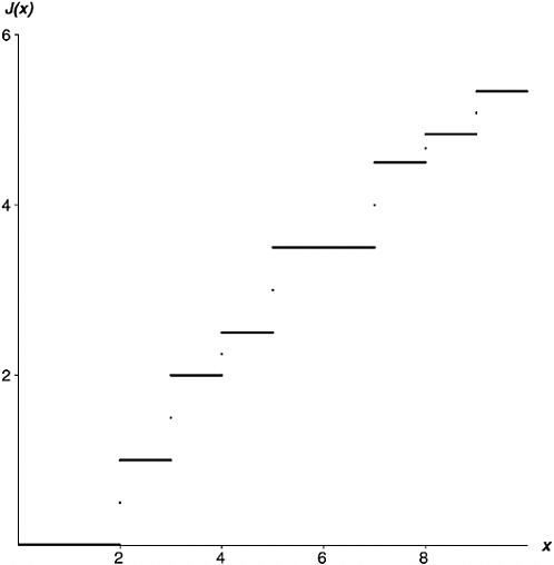
FIGURE 19-2 The function J(x).

If you stare hard at Expression 19-1, you will see the following pattern. First, when x is any prime number, J(x) jumps up 1, because π (x)—the number of primes up to and including x—jumps up 1. Second, when x is the exact square of a prime (e.g., x = 9, which is the square of 3), J(x) jumps up one-half, because the square root of x is a

prime, so jumps up 1. Third, when x is the exact cube of a prime (e.g., x = 8, which is the cube of 2), J(x) jumps up one-third, because the cube root of x is a prime, so jumps up 1. And so on.

Note, by the way, that the J function preserves the feature I introduced with π (x). At the actual point where a jump occurs, the function value is halfway up the jump.

To give a fuller picture of the J function, Figure 19-3 is a graph of J(x) for arguments up to 100. The smallest jump here is at x = 64, which is a sixth power (64 = 2⁶), so the J function jumps up one-sixth at x = 64.

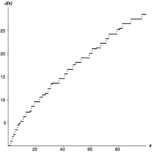
FIGURE 19-3 More of the function J(x).

What possible use is a function like this? Patience, patience. But first, I am going to take one of those leaps I warned you about at the start of the chapter.

IV. I mention yet again that mathematicians have any number of ways to invert relationships. We have an expression for P in terms of Q? OK, let’s see if we can find a way to express Q in terms of P. Over the centuries, mathematics has developed a huge toolbox of inversion tricks, for use in all kinds of circumstances. One of them is called “Möbius inversion,” and it is exactly what we need here.

I’m not going to attempt to explain Möbius inversion in general. Any good textbook on number theory will describe it (see, for example, section 16.4 in Hardy and Wright’s classic Theory of Numbers) and an internet search will turn up numerous references. Rather like the π and J functions themselves, instead of gliding smoothly from one point to the next, I am going to vault over to the following fact: When Möbius inversion is applied to Expression 19-1, the result is as shown in Expression 19-2.

Expression 19-2

You will notice that some terms (the fourth, eighth, ninth) are missing here. Of those that are present, some (the first, sixth, tenth) have a plus sign; others (the second, third, fifth, and seventh) have a minus sign. Anything come to mind? This is the Möbius mu function from Chapter 15. In fact

(where , here and everywhere in the book, is understood to mean just x). Why did you think it was called “Möbius inversion”?

I have now written π (x) in terms of J(x). That is a wonderful thing, because Riemann found a way to express J(x) in terms of ζ (x).

Before leaving Expression 19-2, I’d just like to point out that it is, like Expression 19-1, a finite sum, not an infinite one. This is because the J function, like the π function, is zero when x is less than 2 (check the graph), and if you keep taking roots of a number, the answers eventually drop below 2 and stay there. For example,

which is precisely 25, which is indeed the number of primes less than 100. Magic.

Now let’s turn the Golden Key.

V. Here is the Golden Key, the very first equation in Riemann’s 1859 paper, the one I developed in Chapter 7, arguing that it is just a fancy way to write out the sieve of Eratosthenes.

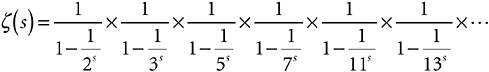
Remember that the numbers on the right-hand side are just primes.

I am going to take the log of both sides. If one thing is equal to another thing, of course its log must be equal to the other thing’s log. From Power Rule 9, which says that log (a × b) = log a + log b,

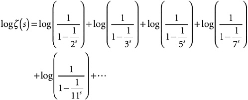
Since by Power Rule 10, this is

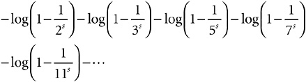
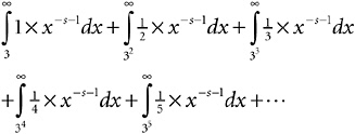
Now recall Sir Isaac Newton’s infinite series for log (1 – x) in Chapter 9.vii. It applied to x between –1 and +1, which is certainly the case here, so long as s is positive. So I can expand each log as an infinite series as shown in Expression 19-3.

Expression 19-3

This is an infinite sum of infinite sums—a bit startling at first sight, I suppose, but not actually an unusual situation in math.

At this point you might think I am much worse off than when I started. From a fairly neat little infinite product, I have now got myself an infinite sum of infinite sums. The situation might seem hopeless. Ah, but that is to reckon without the power of the calculus.

VI. Let me pick on just one term in that sum of sums. I’ll pick on the term . Consider this function: x^–s–1, and assume for the time being that s is a positive number. What’s the integral of x^–s–1? By the general rule for powers, which I gave in Chapter 7.vii, it’s x^–s / (–s), i.e., (–1 / s) × (1 / x^s). If I take the integral at infinity minus the integral at 3², what do I get? Well, if x is a very large number, (–1 / s) × (1 / x^s) is a very small number, so it’s fair to say that when x is infinite, it’s zero. From that—from zero—I’m going to subtract (–1 / s) × (1 / (3²)^s). The answer to this subtraction is (1 / s) × (1 /( 3²)^s). The long and short of it is that the term in Expression 19-3 that I picked on can be rewritten as an integral,

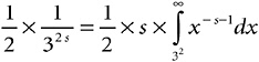
Why in Heaven’s good name would I want to do that? To get back to the J function, that’s why.

You see, x = 3² is where the J function takes a step up of . In a mathematician’s mind—certainly in the mind of a great mathemati

cian like Riemann—that part-expression conjures up an image. The image it conjures up is the one in Figure 19-4. It’s the J function, with a strip filled in. The strip goes from 3² (that is, from 9) to infinity, and it has height one-half. Plainly, the whole area under (“area under”—think “integral”) the J function is made up of strips

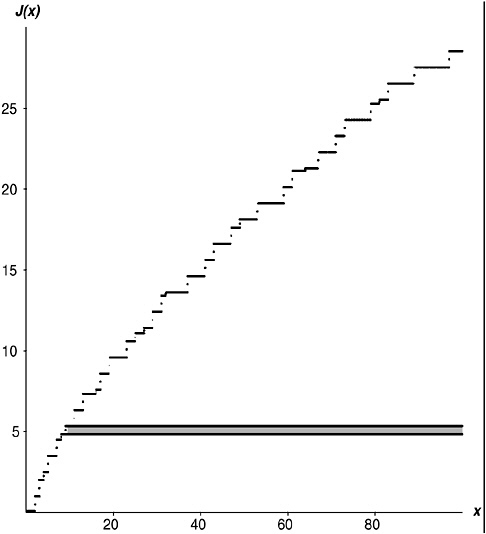
FIGURE 19-4

like that. Strips going from each prime to infinity, with height 1; strips going from each square of a prime to infinity, with height one-half; strips going from each cube of a prime to infinity with height one-third…. See how it all keys in to that infinite sum of infinite sums in Expression 19-3?

Of course, the area under the J function is infinite. The strip I showed has infinite area (height , length infinite, ). So do all the other strips. Together, they add up to an infinity. But what if I were to squish down the J function at the right, so that the area under it is finite? So that each one of those strips tapers away to nothing, with a finite area? How might I accomplish such a squishing-down?

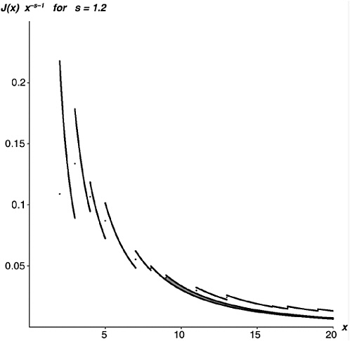
That last integral suggests a way. Suppose I pick some number s (which I shall suppose to be greater than 1). For every argument x, I shall multiply J(x) by x^–s–1. By way of illustration, take s = 1.2. Then x^–s–1 means x^–2.2; or, to put it another way, 1 / x^2.2 . Take an argument x; say, x = 15. Now J(15) has the value 7.333333…; 15^–2.2 has the value 0.00258582…. Multiplying them together, J(x)x^–s–1 has the value 0.018962721…. If I take a bigger argument, the squishing-down is more pronounced. For x = 100, J(x)x^–s–1 has the value 0.001135932….

Figure 19-5 shows a graph of the function J(x)x^–s–1, with s = 1.2. To emphasize the squish-down effect, I have shown the same strip I showed before, now in its squished-down form. You can see how it gets skinnier and skinnier as the arguments head off east. There is a fighting chance that its entire area will be finite, even though it’s infinitely long. Supposing that were true, and supposing it were true of every other strip, what would be the entire area under this function? What, to put it mathematically, would be the value of ?

Let’s see. Taking the primes one by one, for the prime 2 I have, pre-squish, a strip going from 2 to infinity, height 1, then a strip go

FIGURE 19-5 , for s=1.2.

ing from 2² to infinity, height , then a strip going from 2³ to infinity, height , and so on. The sum of the squished strips, considering just the prime 2, is shown in Expression 19-4.

Expression 19-4

Of course, that’s just the 2-strips. There is a similar infinite sum of integrals for the 3-strips, shown in Expression 19-5.

Expression 19-5

There’s another for 5, another for 7, and so on for all the primes. An infinite sum of infinite sums of integrals! Worse and worse! Ah, but things always look darkest before the dawn.

That brings us back to the beginning of this section. Since integration is transparent to a multiplying factor, is the same as 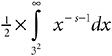. But I showed at the beginning of this section that my sample term from Expression 19-3, , is equal to ; that is, s times the thing I just got. So what does Expression 19-5 amount to? Why, just the second line of Expression 19-3, divided by s! And Expression 19-4, plus Expression 19-5, plus the similar expressions for all the other primes, add up to all of Expression 19-3, divided by s.

Here comes the dawn. It follows that the thing I am currently fooling with, which is 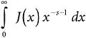, is just Expression 19-3, divided by s. But Expression 19-3 is equal to log ζ (s), from the Golden Key. Hence the result shown in Expression 19-6.

The Golden Key (calculus version)

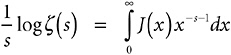
Expression 19-6

I simply cannot tell you how wonderful this result is. It leads directly to the central result in Riemann’s paper, a result I shall show in Chapter 21. Really, it is just a rewriting of the Golden Key in terms of calculus. This is a great and marvelous thing to do, however, as it now opens up the Golden Key to all the powerful tools of nineteenth-century calculus. That was Riemann’s achievement.

One of those tools is yet another inversion method, which allows us to turn this new expression inside out to get an expression for J in terms of ζ . I’m going to hold off showing this inverted expression for the time being. The logic is clear, though.

• I can express π (x) in terms of J(x) (Section IV in this chapter).

• By inverting Expression 19-6, I can express J(x) in terms of the zeta function.

Therefore,

• I can express π (x) in terms of the zeta function.

Which is exactly what Riemann had set out to do, because then all the properties of the π function will be found encoded somehow in the properties of the ζ function.

The π function belongs to number theory; the ζ function belongs to analysis and calculus; and we have just thrown a pontoon bridge across the gap between the two, between counting and measuring. In short, we have just created a powerful result in analytic number theory. Figure 19-6 shows a graphical representation of Expression 19-6, the Golden Key in calculus form.

FIGURE 19-6

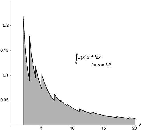
The area shown shaded is , for s = 1.2. Its numerical value is actually 1.434385276163…. This is equal to .