Prime Obsession: Bernhard Riemann and the Greatest Unsolved Problem in Mathematics (2003)

Tom Apostol, Professor of Mathematics Emeritus at Caltech, wrote the following tribute to the Riemann Hypothesis (RH) in 1955 and performed it at the Caltech Number Theory conference held in June of that year. Tom’s original lyrics went only as far as Line 32; the last two stanzas were posted on a bulletin board at Cambridge University in 1973 by algebraic topologist Saunders MacLane.

The song mentions the Lindelöf Hypothesis (LH), a younger cousin of the RH. Dating as it does from 1908, the LH really belongs in Chapter 14 somewhere; but because it is peripheral to the main story, and because it involves the “big oh” notation from Chapter 15, and because I felt that my book already had too much math at that point, I left it out. Tom’s lyrics can’t be understood without it, though, and I couldn’t bear to omit them; so you get a song and a bonus hypothesis!

Where are the zeros of zeta of s?

by Tom M. Apostol

(To the tune of Sweet Betsy from Pike.)

Tune. “Sweet Betsy from Pike” is the song Americans sing to this tune. The tune is older than those lyrics, though. It first showed up attached to an English song popular in the mid-nineteenth century, “Villikens and his Dinah.” (From which, by the way, the cat in Lewis Carroll’s Alice books got its name. “Villikens and his Dinah” was a favorite with Alice Liddell, the girl who inspired the books, and she actually did have a cat named Dinah.) If you had a British education that included membership in a school rugby club, you will most likely recognize the tune as that of the melancholy ballad beginning, “O Father, O Father, I’ve come to confess. I’ve left some poor girl in a hell of a mess….”

Line 1. See Chapter 5.vii.

Line 2. Riemann’s full name was Georg Friedrich Bernhard Riemann (Chapter 2.iii). He seems only ever to have used the “Bernhard.”

Line 3. “Critical line”, see Chapter 12.iii, Figure 12-1.

Line 4. Compare my statement in Chapter 13.viii that at height T up the critical line, the average spacing of zeros is ~ 2π / log(T / 2π ). That means that in a unit length of the line, there are ~ (1 / 2π )log(T / 2π ) zeros. That’s what the songwriter means by “density.” Note that by the rules for logs, log(T / 2π ) is equal to log T – log (2π ), that is, log T – 1.83787706…. If you multiply that by 1 / 2π , you get (1 / 2π )log T – 0.29250721…. As T gets larger and larger, so does log T (albeit much more slowly), and the significance of the 0.29250721… term dwindles to nothing. The density is, therefore, ~ “one over two pi log T.”

Line 8. “ Mod t” refers to the modulus of t, as defined in Chapter 11.v. When, as here, t is understood to be a real number, “mod t”—in proper symbols, “| t |”—just means “the size of t,” that is, t without its sign. | 5 | is 5; | –5 | is also 5. As I pointed out in Chapter 16.iv, “t ” (or “T ”) is pretty standard in zeta-function theory for referring to height up the critical line; or, more generally, as in the discussion of the LH in the notes on Lines 21–28, to the imaginary part of a zeta-function argument.

Line 9. Harald Bohr (Chapter 14.iii) and Edmund Landau proved an important theorem about the S function (see Chapter 22.iv) in 1913. The theorem states that, so long as there is only a finite number of zeta zeros off the critical line, S(t) is unbounded when t goes to infinity. Selberg’s 1946 proof that S(t) is unbounded, which I mentioned in Chapter 22.iv, is stronger, as it does not need that initial condition. For Cramér, see Chapter 20.vii. As well as developing that “probabilistic model” for the prime numbers, Cramér also proved a minor result about the S function: If the LH (see the notes for Lines 21–28) is true, then S(t) / log t dwindles to zero as t goes to infinity. For Littlewood and Hardy, see Chapter 14; for Titchmarsh, see Chapter 16.v.

Lines 13–16. Chapter 14.v.

Line 17. The term “Li” here should be pronounced “ell-eye,” to preserve the meter. The songwriter is here discussing the error term π (x) – Li(x), which I cover extensively in Chapter 21.

Line 18. “The order of P is not known” means, “P is ‘big oh’ of … what? We don’t know.” For big oh, see Chapter 15.ii-iii. By “x high,” the songwriter means, “large values of x.”

Lines 19–20. If we could show that , the RH would follow. That is the converse of von Koch’s 1901 result in Chapter14.viii. I didn’t mention it at the time, but if von Koch’s result is true, the RH follows. Each implies the other.

Lines 21–28. These next few lines are all about the Lindelöf Hypothesis (LH), a famous conjecture in the theory of the zeta function. For Lindelöf the man, see Note 72. His hypothesis concerns the growth of the zeta function in a vertical direction—that is, up a vertical line in the complex plane.

Lindelöf, writing the argument of the zeta function as σ + it, asked: For any given real part σ (that’s a lowercase Greek “sigma,” by the way), what can be said about the size of as t, the imaginary part, goes from zero to infinity? “Size” here means the modulus, as defined in Chapter 11.v; in other words, it means , the distance of the value from zero. This is a real number, so that for any given σ , both the argument t and the value are real numbers. We can therefore draw a graph. Figures A-1 through A-8 show these graphs, for some representative values of σ , and explain the issue better than any number of words.

Note the non-trivial zeros of the zeta function in Figure A-5. Note, in fact, the busyness of Figures A-4 through A-6, compared to the others. With the zeta function, all the interesting action is in the critical strip.

FIGURES A-1 through A-8 for some representative values of σ .

Note also some familiar values when t = 0: in Figure A-4 (corresponding to in Figure 9-3, since of course is just ); infinity, in Figure A-6 (divergence of the harmonic series, Chapter 1.iii); 1.644934 … in Figure A-7 (solution of the Basel problem, Chapter 5.i); and 1.202056 … in Figure A-8 (Apéry’s number, Chapter 5.vi). The function value of zero at t = 0 in Figure A-2 is genuine, a trivial zero (Chapter 9.vi). The apparent zeros in Figures A-1 and A-3 are false; the actual t = 0 values are just too small to register. (They are, respectively, 0.0083333…, and 0.0833333….)

The LH is about finding a big oh (Chapter 15.ii) for these graphs. Just from looking at them, you can guess the following:

• For σ =–1, –2, and –3, the graph looks as if it is big oh of some accelerating function of t, perhaps a power like t² or t⁵, those powers seeming to get bigger as σ heads west along the negative real axis.

• For σ = 2 and 3, it looks as though we are in the world of O(1), or in other words, of O(t ⁰).

• In the critical strip, that is, for σ = 0, , and 1, it is not easy to say what an appropriate big oh might be.

Could it be that, for any value of σ , there is a definite number μ for which ? With μ = 0 when σ is bigger than 1, and μ some increasing positive number when σ goes west from zero? That’s how things look. But then, what happens in the critical strip when σ is between 0 and 1? And in particular, what happens on the critical line when ?

Well, here (see Figure A-9) is what we know for certain at the time of writing. For any given value of σ , there is indeed a number μ for which , for arbitrarily small ε . This is not quite the same as my suggestion in the previous paragraph, but you could be forgiven for ignoring the difference. (If you compare the ε that showed up in Chapter 15.iii, though, you will understand its significance here.) Clearly, this number μ is a function of σ . Hence

FIGURE A-9 Lindelöf’s function.

“the Lindelöf function mu sigma” in Line 22. This is nothing to do with the Möbius μ function of Chapter 15, of course. Here we have another unfortunate case of overloaded symbols.

We also know the following, with mathematical certainty.

• When σ is less than or equal to zero, .

• When σ is greater than or equal to 1, μ (σ ) = 0.

• In the critical strip (that is, when σ is between 0 and 1 exclusive), . In other words, it lies below the dotted line in Figure A-9.

• For all values of σ , μ (σ ) is convex downward. That is, if you join any two points of the graph with a straight line, the arc you cut off lies entirely below, or on, the line. This is true everywhere, including the critical strip; and it implies that for σ between 0 and 1, μ (σ ) must be positive or zero. (Line 26 of the song.)

• The truth of the RH would imply the truth of the LH (which I am just about to state), but not vice versa. The LH is the weaker result.

That, I repeat, is the limit of our current knowledge. The LH, shown in Figure A-10, says that , from which it easily follows

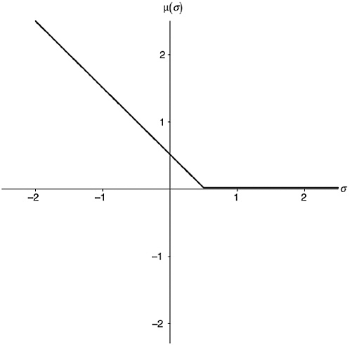
FIGURE A-10 The Lindelöf Hypothesis.

that all the way from negative infinity to , and then is zero for every argument east of that. Compare Lines 27 and 28 of the song. This is an open hypothesis, still unproven. As a matter of fact, we don’t know a single value for μ (σ ) when σ is between 0 and 1, exclusive. The LH is the greatest challenge in zeta-function theory after the RH and has been the subject of intense interest and investigation since Lindelöf stated it in 1908.

Line 24. It can be proved that the LH is equivalent to a statement limiting the number of zeta zeros off the critical line. If the RH is true, of course, there should be no such zeros; but then, as I have already pointed out, if the RH is proved, the LH follows.

Line 31. “In order to strengthen the prime number theorem….” That is, in order to get the best possible big oh expression for the error term.

Line 32. In ordinary integration, as I defined it in Chapter 7.vii, you integrate along the x-axis, from some number a to some bigger number b. In complex variable theory, you integrate along some contour—that is, some line or curve—in the complex plane, from some point on the contour to some other point. Usually, you get to choose the contour. The result might depend on which contour you do your integration along. Contour integration is a key tool in analytic number theory (and in complex function theory generally). To get certain results about the error term, you must integrate along a contour that avoids the zeros.

Line 33. “André Weil….” These last two stanzas refer to the algebraic approach I mentioned in Chapter 17.iii, and to Weil’s 1942 result.

Line 34. “A fancier zeta….” That is, one of those zeta-function analogues associated with finite fields that I mentioned in Chapter 17.iii.

Line 35. “He proves….” Thanks to Weil, we know that the RH-analogy for these special fields is true.

Line 36. I defined the characteristic of a field in Chapter 17.ii. The RH-analogue has been proved only for zeta functions whose associated field has non-zero characteristic—that is, its characteristic is some prime number p.

Line 40. The word “mod” here is being used in the clock arithmetic sense of Chapter 6.viii; as I remarked in Chapter 17.ii, this has connections with field theory.

Among the many alternative versions of Tom’s lyrics to be found on the internet, I note that one ends with the line, “Use R.M.T., and you’ll have better luck.” This is a good-natured dig at the “physical” approach. “R.M.T.” stands for “Random Matrix Theory.”