Prime Obsession: Bernhard Riemann and the Greatest Unsolved Problem in Mathematics (2003)

I. In the last chapter I gave the mathematical background and a little historical background to the Hilbert-Pólya Conjecture. The Conjecture was far ahead of its time and lay there untroubled for half a century.

That was, however, a very eventful half-century in physics, the most eventful ever. In 1917, just around the time of the Conjecture, Ernest Rutherford observed the splitting of the atom; 15 years later, Cockroft and Walton split the atom by artificial means. This led in turn to Enrico Fermi’s work, to the first controlled chain reaction in 1942, and to the first nuclear explosion on July 16, 1945.

“Splitting the atom” is, as all high-school physics teachers tell their classes, a misnomer. You split atoms every time you strike a match. What we are really talking about here is the splitting of the atomic nucleus, the heart of the atom. To get a nuclear reaction— controlled or otherwise—going, you must fire a subatomic particle into the nucleus of a very heavy element. If you do that in a certain way, the nucleus splits, firing off new subatomic particles as it does. These particles penetrate the nuclei of neighboring atoms … and so on, leading to a chain reaction.

Now, the nucleus of a heavy element is a very peculiar beast. You can visualize it as a seething, wobbling blob of protons and neutrons, welded together in such a way that it’s hard to say where one particle starts and another ends. In the case of seriously heavy elements like uranium, the whole blob is teetering on the edge of instability. It might, in fact, depending on the precise mix of protons and neutrons, be actually unstable, liable to fly apart of its own volition.

As nuclear physics developed through the middle decades of the twentieth century, it became very important to understand the behavior of this strange beast and, in particular, to understand what happens if you fire a particle into it. Now, this nucleus, this wobbling blob, can exist in a number of states, some having high energy (imagine really energetic wobbling), some having low energy (a dull, languorous kind of wobbling). If a particle is fired into it so that the nucleus absorbs the particle instead of flying apart, then—since the energy of the particle must go somewhere—the nucleus moves from a lower state of energy to a higher. Later, tired of all the excitement, it might eject an equivalent particle, or perhaps a different type of particle altogether, and resume a lower energy state.

How many possible energy levels are there? When does a nucleus pass from level a to level b? How are the energy levels spaced relative to each other, and why are they spaced like that? Questions like these placed the study of the nucleus in a larger class of problems, problems about dynamical systems, collections of particles each of which has, at any point in time, a certain position and a certain velocity. As investigations proceeded through the 1950s, it became apparent that some of the most interesting dynamical systems in the quantum realm, including the heavy nucleus, were too complicated to yield to exact mathematical analysis. The number of energy levels was too large, the possible configurations too numerous. The whole thing was a nightmare version of the “many-body” problem of classical (that is, pre-quantum) mechanics, where several objects—the planets of the solar system, for example—are all acting on each other through gravity.

Precise mathematics has trouble coping with this level of complexity, so investigators fall back on statistics. If we can’t discover exactly what’s going to happen, perhaps we can discover what, on average, is most likely to happen. Such statistical approaches had been extensively developed in classical mechanics, beginning as far back as the 1850s, long before quantum theory appeared. Things go somewhat differently in the quantum world, but at least there was a good body of classical theory to provide inspiration. The necessary work was done, the necessary statistical tools for complex quantum dynamical systems like heavy-element nuclei were developed in the late 1950s and early 1960s, key players being the nuclear physicists Eugene Wigner and Freeman Dyson. One central concept was that of a random matrix.

II. A random matrix is just what its name suggests, a matrix made up of numbers chosen at random. Not quite at random, actually. Let me offer an illustration. Here is a random 4 × 4 matrix, of a rather particular type whose relevance I shall explain later. I round everything to four places of decimals in what follows, to save space.

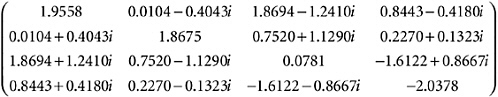
The first thing you may notice about this contraption is that it is Hermitian—it has that not-quite-symmetry about the lead diagonal that I described in Chapter 17.v. Recall the following facts from that chapter.

• Associated with every N × N matrix is a polynomial of degree N, called the characteristic polynomial.

• The zeros of the characteristic polynomial are called the eigenvalues of the matrix.

• The sum of the eigenvalues is called the trace of the matrix (and is equal to the sum of the lead-diagonal elements).

• In the particular case of a Hermitian matrix, the eigenvalues are all real and so, therefore, are the coefficients of the characteristic polynomial, and also the trace.

For the sample matrix I have shown here, the characteristic polynomial is

The eigenvalues are: – 3.8729, 0.0826, 1.5675, and 4.0864. The trace is 1.8636.

Now turn your attention to the actual numbers that make up that sample matrix. The numbers you see there—the real numbers that make up the lead diagonal (with a slight qualification, see below), and all the real parts and imaginary parts of the off-diagonal complex numbers—are random in a certain special sense. They are plucked at random from a Gaussian-normal distribution—the famous “bell curve” that crops up all over the place in statistics.

Imagine the standard bell curve drawn on a sheet of fine-ruled graph paper, so that there are hundreds of graph-paper squares under the curve (Figure 18-1). Pick one of those squares at random; its horizontal distance from the peak center-line is a Gaussian-normal random number. There are many more of those squares clustered round the peak than there are out in the tails of the curve so you are much more likely to get a number between –1 and +1 than you are to get a number to the right of +2, or to the left of –2. So you see if you look at the numbers in the sample matrix shown at the beginning of this section. (Though the lead-diagonal elements are actually Gaussian-normal random numbers multiplied by for technical reasons, and are, therefore, a bit bigger than you would expect.)

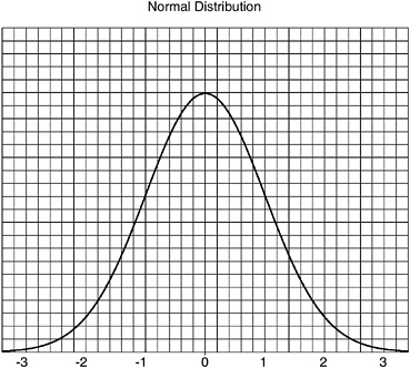
FIGURE 18-1 The Gaussian-normal distribution.

Gaussian-random Hermitian matrices like that one, though much, much bigger, proved to be just the ticket for modeling the behavior of certain quantum-dynamical systems. In particular, their eigenvalues turned out to provide an excellent fit for the energy levels observed in experiments. Therefore these eigenvalues, the eigenvalues of random Hermitian matrices, became the subject of intensive study through the 1960s. Their spacing in particular turned out to be very interesting. They were not spaced at random. It was, for example, much more unusual than you would expect, on a random basis, for two levels to be close to each other. This is the phenomenon called “repulsion”—energy levels trying to get as far as possible from each other, like a long standing line of antisocial people.

To give you a visual aid to what I am describing here, I asked my math software package, Mathematica 4, to generate a random 269 × 269 Hermitian matrix and compute its eigenvalues (see Figure 18-2).

The reason for using the number 269 here will become clear very shortly. Mathematica, which never ceases to amaze me, did this in a trice. The 269 eigenvalues ranged from –46.207887 to 46.3253478. My idea was to string them out as blobs on a line going from –50 to +50, like raindrops on a fence wire, to show you the pattern of spacings. There was no way I could fit this neatly on a book page, though; so I chopped up the line into 10 equal segments (–50 to –40, –40 to –30, and so on) and just stacked the segments on top of each other to make Figure 18-2.

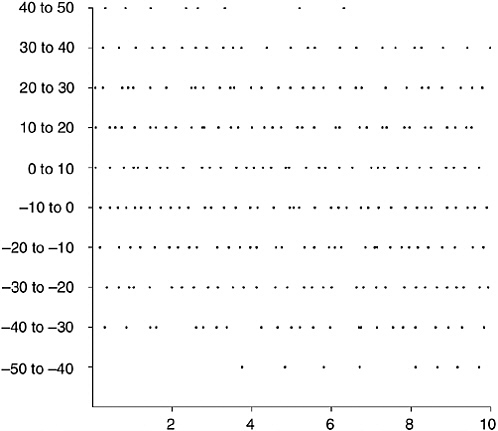
FIGURE 18-2 The eigenvalues of a 269-by-269 random Hermitian matrix.

There is no obvious pattern to the spacing. You might say that it is random. Not at all! Figure 18-3 shows 269 numbers picked entirely at random in the range 0–10 and plotted in the same way. Comparing Figures 18-2 and 18-3, you can see that the eigenvalues of a random matrix are not randomly scattered across their range. You can see the

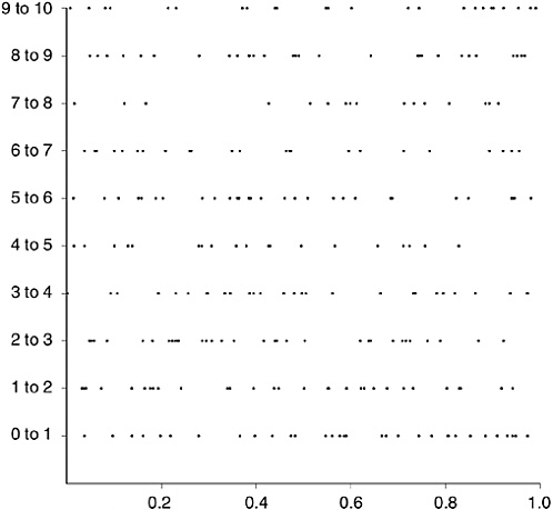
FIGURE 18-3 Random spacings: 269 random numbers between 0 and 10.

repulsion effect in Figure 18-2—the random scattering of Figure 18-3 has more adjacent pairs of values very close together than has the eigenvalue distribution (and, inevitably, more far apart, too). The eigenvalues in Figure 18-2, though unwilling to form any recognizable patterns—they arise, after all, from a random matrix—are struggling to keep their distance from each other. A purely random dot, by contrast, doesn’t seem to mind at all if it finds itself jammed up against another random dot.

Permit me to introduce three terms of art here. The set of random (that is, Gaussian-random) Hermitian matrices¹⁰³ of the type I have been describing is called, in its totality, the “Gaussian Unitary Ensemble,” or GUE (pronounced “goo”). The precise statistical prop-

erties of the spacings between a long non-uniform string of numbers like those I have illustrated are encapsulated in a creature called the “pair correlation function.” And a certain ratio associated with this function, and highly characteristic of it, is called its “form factor.”

Now I am in a position to tell you about a remarkable meeting, one that opened up very strange and mysterious questions about the Riemann Hypothesis and launched a thousand research projects.

III. The meeting, a chance encounter between a number theorist and a physicist, occurred at Princeton’s Institute for Advanced Study in the spring of 1972. The number theorist was Hugh Montgomery, a young American doing graduate work at Trinity College, Cambridge—G.H. Hardy’s old college. The physicist was Freeman Dyson, who held a professorship at the Institute. Dyson, whom I mentioned earlier, was a renowned physicist. He had not yet embarked on his second career as an author of thought-provoking bestsellers about the origins of life and the future of the human race.

Hugh Montgomery’s most recent work had been an investigation of the spacing between non-trivial zeros of the zeta function. This was not part of any attempt to prove the Riemann Hypothesis. It just happens that a result about the nature of that spacing has consequences in the theory of number fields, fields somewhat like the field that I showed you in Chapter 17.ii.¹⁰⁴ This was Montgomery’s area of interest. Here is the story as he tells it.

You can understand why Freeman Dyson was so excited. The expression that Hugh Montgomery mentioned, the expression that had emerged from his inquiries into the Riemann zeta function’s non-trivial zeros, was precisely the form factor associated with a random

Hermitian matrix—the kind of thing Dyson had been involved with for several years in his researches into quantum dynamical systems. (And Montgomery even understated the degree of serendipity involved in this meeting. Though he made his name as a physicist, Dyson’s first degree was in math, and his first area of interest was number theory. If this had not been so, he might not have grasped what Montgomery was talking about.¹⁰⁸)

To illustrate the point, I am going to take all the non-trivial zeros of the Riemann zeta function up to the height 500i—that is, on the critical line (they all are on the critical line; the Riemann Hypothesis is certainly true down at these low levels)—from to . There are 269 zeros in this range. (That is why I picked the number 269 for Figures 18-2 and 18-3.) Figure 18-4 shows them, their range chopped into 10 segments and stacked up just as before. If you compare this with Figures 18-2 and 18-3, you see that it resembles Figure 18-2, not Figure 18-3.

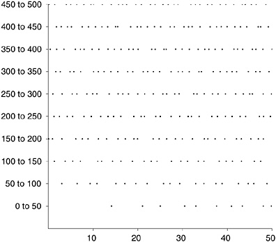
FIGURE 18-4 The first 269 values of “t,” where is a non-trivial zero of the zeta function.

You should make some modest allowances when comparing these figures. The zeta zeros in Figure 18-4 take a while to get started and pack closer further up the critical line, according to the principle I stated in Chapter 13.viii. Also, the eigenvalues in Figure 18-2 are stretched out somewhat at the beginning and end of their range and correspondingly squished in the middle. Both effects can be reduced by taking more zeros and bigger matrices and by normalizing (see below). Even allowing for these distortions, the following points look pretty plausible on the basis of these diagrams.

• Neither the zeta zeros nor the eigenvalues look much like randomly scattered points.

• They resemble each other.

• In particular, they both show the repulsion effect.

IV. Hugh Montgomery’s paper on the spacing of zeta zeros was published by the American Mathematical Society in 1973. Its first words are, “We assume the Riemann Hypothesis (RH) throughout this paper….” There is nothing very striking about that. By 1973 a vast amount of mathematical literature consisted of theorems that assumed the truth of the Hypothesis.¹⁰⁹ Today the quantity is correspondingly vaster, and if the RH (as I shall henceforth term it, following Montgomery and all other modern researchers) proves false, this entire superstructure will become unstable; though if the counterexamples are few, much could be rescued.

Montgomery’s 1973 paper contains two results. The first is a theorem about the broad statistical properties of the zeta-zero spacing. This theorem presupposes the truth of the RH. The second result is a conjecture. It asserts that the pair correlation function for the spacing is what Montgomery told Dyson he thought it was. It is important to understand that this is a conjecture. Montgomery was not

able to prove it, not even on the assumption that the RH is true. Nobody else has been able to prove it, either.

Most of the features of the Riemann zeros that you will see reported and discussed, most of the ideas that have come up in the last 30 years, are likewise conjectural. Hard proofs are in desperately short supply in this area. In part this is because, following the link established by Montgomery, so much of the recent thinking about the RH has been done by physicists and applied mathematicians. Sir Michael Berry¹¹⁰ likes to quote the Nobel Prize-winning physicist Richard Feynman in this context, “A great deal more is known than has been proved.” In part it is also because the RH is a very, very tough problem. There is such an immense quantity of literature on the RH now that you have to keep reminding yourself of the truth that very little is known for certain about the zeros of the zeta function, and even with all the rising interest during the past few years, results that are mathematically watertight still come only occasionally, at long intervals.

V. The Institute for Advanced Study in Princeton, New Jersey, is only 32 miles from AT&T’s Bell Labs research center in Murray Hill. Hugh Montgomery lectured on what was, by that time, the “Montgomery pair correlation conjecture” at Princeton in 1978. Among those present was Andrew Odlyzko, a young researcher from the AT&T facility. At just about this time, his laboratory acquired a Cray-1 supercomputer. Researchers were encouraged to run projects on the Cray, to familiarize themselves with the kinds of algorithms appropriate to its architecture.

Ruminating on Montgomery’s lecture, Odlyzko reasoned as follows. The Montgomery conjecture asserts that the spacing of zeta zeros follows such-and-such a statistical law. This law also appears in the investigation of a certain family of quantum dynamical systems that conform to the GUE model. The statistical properties of that

family have been the subject of intensive analysis over several years. The statistical properties of the zeta zeros, however, have been very little investigated. Useful work could be done, the balance redressed, by undertaking a statistical study of the zeta zeros.

That is what Andrew Odlyzko proceeded to do. Using spare time in 5-hour segments on the Cray computers¹¹¹ at Bell Labs, he generated the first 100,000 non-trivial zeros of the Riemann zeta function to high accuracy (around 8 decimal places), using the Riemann-Siegel formula. Then, to get a snapshot of the situation much higher up the critical line, he generated another 100,000 zeros starting with the 1,000,000,000,001st. He then ran these two sets of zeros through various statistical tests, to see how they compared with the eigenvalues of matrices for GUE operators. The results of all this work were published in a landmark paper in 1987, under the title, “On the Distribution of Spacings Between Zeros of the Zeta Function.”

The results were not quite conclusive. As Odlyzko put it very delicately in the paper, “The data presented so far are fairly consistent with the GUE predictions.” There were slightly more small spacings than the GUE model predicted. Odlyzko’s results were sufficiently impressive, though, to capture the attention of a wide range of researchers. Further work cleared up the discrepancies noted in the 1987 paper, and the Montgomery Pair Correlation Conjecture became the Montgomery-Odlyzko Law.¹¹²

The Montgomery-Odlyzko Law

The distribution of the spacings between successive non-trivial zeros of the Riemann zeta function (suitably normalized) is statistically identical with the distribution of eigenvalue spacings in a GUE operator.

VI. I can give only a brief sketch of the nature of Odlyzko’s results. To do so, I duplicated them on my own PC, using a list of the zeros

that Odlyzko has helpfully posted on his web site. To avoid any startup anomalies, I took the 90,001st to the 100,000th zeros, counting up the critical line from . That’s 10,000 zeros—quite sufficient to make some statistical sense of. The 90,001st zero is at ; the 100,000th is at (rounding to 4 decimal places). I am thus going to investigate the statistical properties of a sequence of 10,000 real numbers, a sequence that starts with 68194.3528 and ends with 74920.8275.

Since, as I pointed out in Chapter 13.viii, the zeros get closer together, on average, as you go up the critical line, I must make an adjustment to stretch out the higher end of this range. This I can do quite simply by multiplying every number by its log. Bigger numbers have bigger logs, and this is just what I need to even out the average spacing. This is the meaning of the word “normalized” in the statement of the Montgomery-Odlyzko Law given above. My sequence now begins with 759011.1279 and ends with 840925.3931.

Furthermore, I am interested in the relative spacing of the zeros; so I can subtract 759011.1279 from every number in the sequence without affecting my result. The sequence now goes from zero to 81914.2653. Finally, just to make the numbers neater, I am going to switch to a different scale, dividing every number in my sequence by 8.19142653. Again, this doesn’t affect the relative spacing; I have merely switched rulers. This final form of my sequence starts like this: 0, 1.2473, 2.5840, …, and ends like this: 9997.3850, 9999.1528, 10,000.

If you include the end points, I now have 10,000 numbers laid out for study, ranging from 0 to 10,000. Since there are 9,999 spaces between consecutive numbers, the average spacing is 10,000 ÷ 9,999, which is just a shade greater than 1.

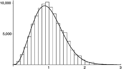
FIGURE 18-5 The Montgomery-Odlyzko Law. (Distribution of spacings for the 90,001st to 100,000th zeta-function zeros.)

Now I can ask statistical questions. Sample question: How do the spacings depart from that average? How many have a length less than one?¹¹³ The answer is 5,349. How many have a length of more than 3? None. Now, this is at total variance with the counts you get from a perfectly random scattering, which are 6,321 and 489, respectively.¹¹⁴ That confirms the lesson of Figures 18-2 and 18-3. The zeros are not randomly scattered. They are more bunched around the average spacing (a tad more than 1), with a dearth of small spacings and a dearth of large ones.

Tallying the number of spacings with length between 0 and 0.1, between 0.1 and 0.2, and so on, and making a histogram of the tallies, scaled so that the whole area is 9,999, I get Figure 18.5. This shows the spacings for my 10,000 zeros against the curve predicted by GUE theory. It’s not a sensationally good fit, but then my sample isn’t very big, or very high up the critical line. The fit is good enough, well within the variation allowed by chance; and the fits in Andrew Odlyzko’s paper are of course much better.¹¹⁵

VII. So yes, it seems that the non-trivial zeros of the zeta function and the eigenvalues of random Hermitian matrices are related in some way. This raises a rather large question, a question that has been hanging in the air ever since that encounter in Fuld Hall in 1972.

The non-trivial zeros of Riemann’s zeta function arise from inquiries into the distribution of prime numbers. The eigenvalues of a random Hermitian matrix arise from inquiries into the behavior of systems of subatomic particles under the laws of quantum mechanics. What on earth does the distribution of prime numbers have to do with the behavior of subatomic particles?