
Hydroacoustic Considerations in Marine Propulsor Design
M.Sevik (David Taylor Model Basin, USA)
ABSTRACT
Hydroacoustics is based on firm theoretical foundations which overlap with those of aeroacoustics. Hydroacoustics is characterized by low Mach numbers, a high impedance relative to air, and important fluid loading effects on submerged structures. Fluid flow fields affecting marine propulsors are unsteady and give rise to time-dependent pressures which excite internal and adjacent external structures into vibrations. In the absence of cavitation, dipole sources on stationary and rotating blade rows of ship propulsors are the dominant contributors to the acoustic far field. When located in an elastic enclosure, the near-field of dipoles close to the blade tips excite the structure which adds additional energy to the sound field. The combined levels and directivity patterns are different from those of an open propeller in free-field. At this time, the complex flow fields and the response of structures cannot be reliably predicted by numerical techniques. Large, quiet, high speed water tunnels have been equipped with acoustic arrays in order to provide a preliminary assessment of the performance of alternative propulsor designs.
HISTORICAL REMINDERS
The study of flow-induced noise was stimulated in the early fifties when airliners powered by jet engines entered the commercial market. A fundamental paper which explained the physics of sound generation by turbulence was published by Lighthill(1) in 1952. In the same time-frame, pioneering work by Powell(2), Ffowcs Williams(3) and Curle(4) provided insights which paved the way for future progress.
At a symposium dedicated to hydrodynamics, it is appropriate to recall that the wave equation is derived from the familiar equations of momentum and continuity. Since sound is a very weak disturbance to a fluid at rest, viscosity can be ignored and motions can be restricted to vanishingly small values. The fluctuations of density ρ and pressure p vary little about their mean values. Away from the turbulence, both satisfy the homogeneous wave equation
ò2ρ/òt2–c2 ![]() 2ρ=0 (1)
2ρ=0 (1)
If fluid or momentum is created in a region, a function Q(x,t) representing the acoustic source density is added to the right hand side. If an external force Fi acts on the fluid, Q (x,t) has the form of a divergence òFi/òxi. For turbulence, Q(x,t) is a double divergence and the inhomogeneous wave equation has the form
ò2ρ/òt2–c2 ![]() 2 ρ=ò2Tij/òxiòxj (2)
2 ρ=ò2Tij/òxiòxj (2)
Solutions of these basic equations which satisfy various boundary conditions have provided the major tools of noise control.
SOUND RADIATION FROM WATERBORNE VEHICLES
The sound radiated by waterborne vehicles which are propelled at moderate to high speeds involves complex interactions between fluid dynamics and structural acoustics. Cavitation is avoided by the designers whenever radiated noise requirements are imposed and will not be considered in this paper. The remaining problem of radiated noise control involves flow fields that are spatially and temporally random. All structures within such flows are compliant and respond dynamically to time-dependent pressures. The sound field is therefore caused by vibrations and by fluctuating pressures on various surfaces. Mathematically, the acoustic density fluctuations at x in the fluid due to a normal velocity v and a pressure p at a point y on the surface S have been expressed by Ffowcs Williams(5) in the form:
ρ=(1/4πc2x) ò/òt ∫s ni{ρovi+(xi/x)(p/c)} (y,t–|x–y|c–1)dy (3)
In most marine applications, the flow velocity is much smaller than the speed of sound. Typical Mach numbers are on the order of 10–2. Under these conditions length scales of flow or boundary fluctuations are usually compact on an acoustic wavelength scale and retarded time changes are negligible. Dimensional analysis yields simple expressions for the density fluctuations. For example, the first term under the integral sign is due to small amplitude motions of the surface S. If this motion is induced by a flow of velocity U and length scales L, the frequencies will be of the order U/L and
ρ2 ~ ρo2 U4 L2 {c4x2}–1 (4)
The second term under the integral sign is due to pressure fluctuations which may be caused by flow or structural vibrations. Dimensional analysis yields:
ρ2~ρ02U6L2{c6x2}–1 (5)
This dependence on the sixth power of the flow is characteristic of dipoles on a compact scale. However, even at the low Mach numbers prevailing in underwater acoustics, sources are not always compact and consequently a different speed dependence will apply.
Generally, the flow is not affected by structural vibrations since the amplitudes are much smaller than the characteristic length scales of the fluid. An exception is the well-known phenomenon of propeller “singing” where blade vibrations tend to increase the coherence of a periodically shed vortex wake which, in turn, feeds more energy into the structure.
At moderate to high speeds, the propulsor is the most important contributor to a vehicle's radiated noise. The major sources are due to the following effects:
-
The response of rotating blade rows to flow disturbances caused by upstream hydrofoils, such as stator vanes, control surfaces and other fixed appendages. The radiation consists of tonals at blade passage frequencies whose amplitudes are randomly modulated, as shown in Fig. (1).
-
The response of stationary or rotating blade rows to ingested turbulence which may be generated on the hull of the vehicle.
-
The response of rotating blade rows to self-generated flow distortions, as shown in Fig. (2) and of stators located downstream.
-
The scattering of boundary layer turbulence from trailing edges.
-
Radiation from structures which are coupled to the propulsor through hydrodynamic, acoustic and structural paths.
An authoritative treatise covering these topics is provided by Blake (6) in “Mechanics of Flow-Induced Sound and Vibration”.
SOME CASE HISTORIES
In the mid-sixties, the fluctuating thrust of open propellers subjected to a turbulent inflow was of interest. A study of this problem was reported by Sevik(7) at the Seventh Symposium on Naval Hydrodynamics. Experiments were performed in the Water Tunnel at the Applied Research Laboratory of the Pennsylvania State University. Its test section has a diameter of 1.22 m and a length of 4.27 m. The advantage of this facility is that relatively large propellers can be tested at high Reynolds numbers. Fig. (3) shows the installation of a ten bladed propeller in the test section. It had a diameter of 20.3 cm and its chord length was 2.54 cm. The fluctuating thrust was measured with a high impedance dynamometer which had a linear response over the frequency range of interest.
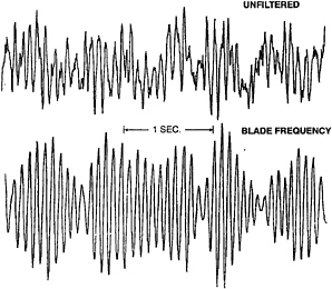
FIG. 1 ACOUSTIC LEVELS AT BLADE RATE FREQUENCY (FROM STRASBERG)
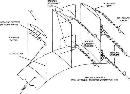
FIG. 2 FLOW FIELD IN A ROTATING BLADE ROW (FROM LAKSHMINARAYANA AND HORLOCK)
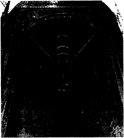
FIG. 3 FREE-STREAM PROPELLER AND BALANCE HOUSING MOUNTED IN THE WATER TUNNEL TEST SECTION
In order to simplify the interpretation of the data, an attempt was made to generate the simplest form of turbulence possible. For this purpose, two grids were installed sequentially upstream of the propeller, as shown in Fig. (4). The mesh sizes were 10.2 and 15.2 cms, respectively. The results of the experiment are shown in Figs. (5) and (6). The principal features of the data are as follows:
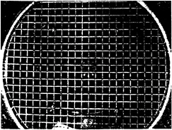
FIG. 4 PROPELLER AS SEEN THROUGH A 4-INCH GRID UPSTREAM OF THE PROPELLER
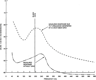
FIG. 5 POWER SPECTRAL DENSITY OF THE RESPONSE OF A TEN-BLADED, 8-INCH-DIAMETER PROPELLER TO TURBULENCE DISTANCE BETWEEN THE GRID AND THE PROPELLER=20 M=80 INCHES; MEASURED WATER-TUNNEL TURBULENCE LEVEL WITHOUT THE GRID U=0.0011U; TURBULENCE LEVEL AT THE PROPELLER DUE TO THE GRID U=0.03U; TUNNEL VELOCITY U=15.4 FT/SEC; PROPELLER ADVANCE RATIO J=1.22)
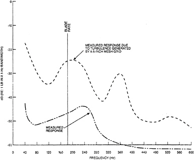
FIG. 6 POWER SPECTRAL DENSITY OF THE RESPONSE OF A TEN-BLADED, 8-INCH-DIAMETER PROPELLER TO TURBULENCE DISTANCE BETWEEN THE GRID AND THE PROPELLER=20 M=120 INCHES; MEASURED WATER-TUNNEL TURBULENCE LEVEL WITHOUT THE GRID U=0.0011U; TURBULENCE LEVEL AT THE PROPELLER DUE TO THE GRID U=0.03U; TUNNEL VELOCITY U=15.1 FT/SEC; PROPELLER ADVANCE RATIO J=1.22)
-
“humps” of energy are superimposed on a broadband spectrum;
-
the humps peak at a frequency slightly higher than the blade rate frequency.
An understanding of these observations has been provided in recent papers by Jiang et al(8), by Martinez(9) as well as, earlier, by Blake. Basically, the propeller acts as a spatial filter: at any instant of time, it responds preferentially to all circumferential wavelengths of the turbulence that are integral numbers of the blade spacing. Most analytic formulations are therefore based on a wavenumber decomposition of the turbulence. Using this approach, Martinez successfully explained the major features of the experimental results. Jiang et al chose a “correlation” approach and used the classical equations for the longitudinal and lateral velocity correlations for homogeneous and isotropic turbulence. The longitudinal correlation function is expressed as an exponential
f(r)=e–r(τ)/Λ (6)
where Λ is the integral scale of the turbulence.
r(τ) accounts for the free stream velocity V, for the rotational speed of the propeller Ω and for the distance between points α and β located on the propeller. It is of the form:
r(τ)2=(Vτ)2+rα2+rβ2+2rαrβ cos(θα–θβ+Ωτ) (7)
The results of this analysis are plotted in Figs. (7) and (8). As before, the theory predicts the major features of the measured data. The theories of Jiang and Martinez are general and apply to all correlation lengths and frequencies. The directivity of the sound field corresponds to that of a compact dipole.
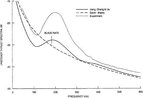
FIG. 7 COMPARISON OF THEORY AND EXPERIMENT (FROM REF. 8)
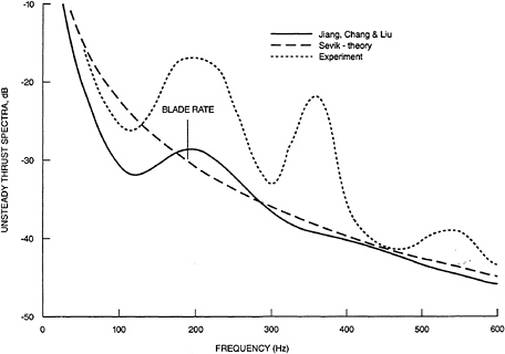
FIG. 8 COMPARISON OF THEORY AND EXPERIMENT (FROM REF. 8)
For clarity, the major design parameters which affect the response of a rotor will be given for small and large correlation lengths of the turbulence. Equations for the mean square value of the unsteady thrust are given by Blake. From these, the mean square value of the density fluctuations depends upon the following parameters:
ρ2 ~ (U/c)6 (u/U)2 [S(ωb/U)]2 F[Λm B/R]2 {As (2πω/B Ω)}2 (8)
where U=the resultant velocity at the tip of the blades, B=the number of blades, S denotes an unsteady hydrodynamic response function (b= chord/2), As=the spatial filtering function of the propeller.
For large correlation lengths, the function {As}2 =B2 for f/ns=mB, where f=frequency and ns is the shaft rotation velocity Ω/2π. The corresponding bandwidth is Δf=ns.
Small correlation lengths occur when the axial scale 2Λ is much smaller than the blade spacing projected in the axial direction. In this case {As}2=1 and each blade responds to the flow independently of the others. Fig. (9) extracted from Blake, illustrates the spectra of the fluctuating thrust for small and large correlation lengths.
Clearly, the propulsor designer will prefer an inflow containing low levels of turbulence and small correlation lengths. Subject to additional requirements such as propulsive efficiency and cavitation, he will select a low blade tip speed and a hydrofoil geometry which is non-responsive to upstream flow fluctuations. Normally, these conditions are difficult to meet.
In some turbomachinery applications, rotors may be located within an elastic enclosure of finite length. The nearfield of the sources at the tips of the blades apply unsteady pressures on the enclosure which is set into vibrations and radiates sound. A recent paper by Kim(10) illustrates this effect for cases of dipole sources at the tips.
The problem considered is shown in Fig. (10). A free-flooded cylindrical shell is excited by a radial force. The governing equation whose simultaneous solution is required are given in Fig. (11). As a specific illustration, Kim analyzed a steel shell submerged in water. For each axial mode m, the
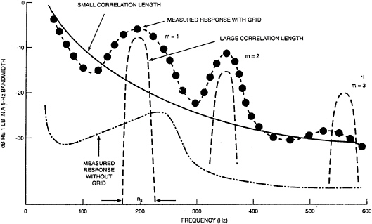
FIG. 9 SPECTRUM (Δf=1 Hz BAND) OF UNSTEADY THRUST ON A 10-BLADED ROTOR DOWN-STREAM OF A 6-IN. GRID WIRE SCREEN FOR WHICH THE MEASURED ΔΘ=0.5RT, RT=4 IN., ns=19 REV/MIN. (ADAPTED FROM SEVIK [146].) (FROM REF. 6)
response of the cylinder for various circumferential N modes are calculated. Resonances appear as “beads” in Figs. (12) to (15). These figures show the amplitudes of forced accelerance of the shell (in color) as a function of both circumferential mode order and frequency. The farfield acoustic pressure for the same shell whose length to diameter ratio is equal to one is shown in Fig. (16). The nearfield patterns for this shell in Fig. (17) indicate intense regions of radiation near the point of application of the radial force as well as at the ends of the cylinder where flexural waves are scattered and launch acoustic energy into the farfield. This effect is also evident in Fig. (18) for a somewhat larger shell (L/a=3). In this case, however, the contribution from the region of the drive point is relatively more pronounced. Kim's example demonstrates that the sound field generated by a blade row encased in an elastic shell has a complex directivity pattern, quite different from that of a dipole.
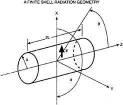
FIG. 10 FREE-FLOODED SHELL EXCITED BY A POINT FORCE (FROM KIM)
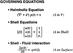
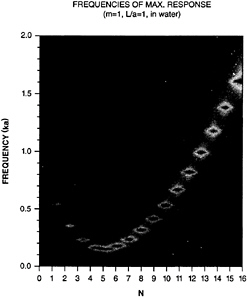
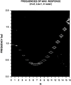
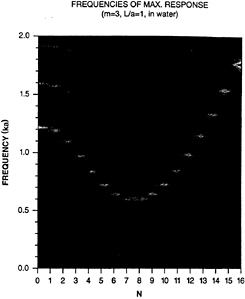
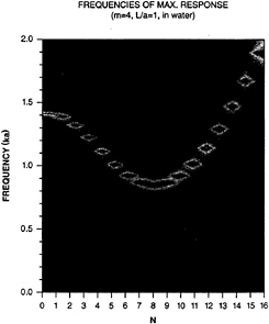
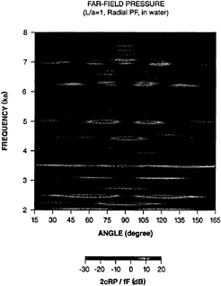
FIG. 16 WHERE P IS THE PRESSURE AT DISTANCE R (FROM KIM) REF. 10
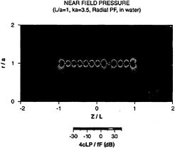
FIG. 17 (FROM KIM) REF. 10
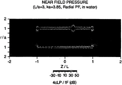
FIG. 18 (FROM KIM) REF. 10
A method for noise mitigation has been suggested by Howe(11). He considered the effects of a pressure-release coating of finite extent installed on an elastic plate located adjacent to hydroacoustic dipole sources. He predicted the influence of the coating on the sound radiated by the dipoles and on the vibrations of the plate.
His analysis involves longitudinal dipoles oriented parallel to the plate, as they would be on the tips of an enclosed blade. The effect of the pressure-release material is to produce equal and opposite images which reduce the efficiency of radiation to quadrupole sources.
Fig. (19) illustrates the model analyzed. For a steel plate of thickness h in water, the radiated sound level and the plate response are plotted as a function of the applied to the coincidence frequency. For values of d/h <5, Fig. (20) illustrates the excess sound scattered by the edge of the coating due to its proximity to the dipole and its ability to extract energy from its nearfield. However, when the coating extends approximately 10-plate thicknesses beyond the location of the dipole, very significant reductions in radiated sound power can be achieved, except at frequencies near coincidence.
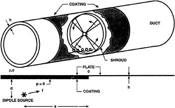
FIG. 19 BLADE-VORTEX INTERACTIONS IN A DUCT CONSIDERED BY HOWE (FROM-REF. 11)
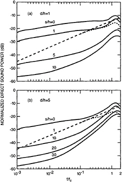
FIG. 20 SOUND POWER FOR A STEEL PLATE AS A FUNCTION OF APPLIED TO COINCIDENCE FREQUENCY FOR:
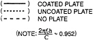
(FROM REF. 11)
HYDROACOUSTIC TEST FACILITIES
In spite of considerable progress, current numerical techniques are not able to predict reliably the complex flow fields and time-dependent interactions which occur on the blades and nearby structures of modern propulsors. Hydroacoustic test facilities—specifically large, quiet, high speed water tunnels—are essential tools for assessing the hydrodynamic and hydroacoustic performance of alternative designs.
The two principal facilities in the United States are the Large Cavitation Channel (LCC) of the Naval Surface Warfare Center, located in Memphis, Tennessee, and the 48-inch Water Tunnel of the Applied Research Laboratory (ARL), at the Pennsylvania State University, in State College, Pennsylvania. These facilities contain complementary and mutually supportive capabilities.
Fig. (21) shows the installation of two sets of acoustic sensors in the LCC, one in an anechoically treated trough under the test section and a second located in the main diffuser section. This arrangement allows a model to be acoustically scanned along its beam aspect and also measured at stern aspect with the acoustic lens. Details of the nested arrays are shown in Figs. (22) and (23). The general design features of the acoustic lens are provided in Fig. (24). Table (I) lists the frequencies and beam widths of the various acoustic sensors. Under non-cavitating conditions, useful data can be acquired up to 80kHz, depending on the characteristics of the test object. The omniphones give an early warning of incipient cavitation. The measured self noise levels of the nested arrays as a function of tunnel speed are given in Fig. (25).
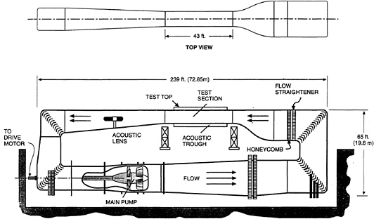
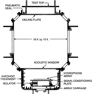
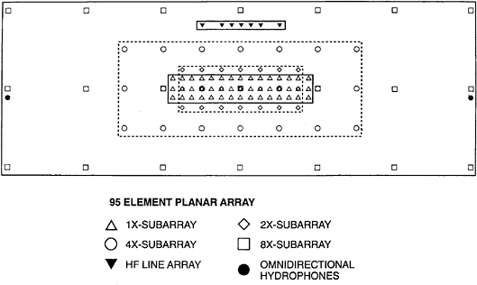
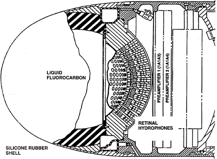
TABLE I: LCC ACOUSTIC SENSORS
|
SubArray |
Design Frequency (kHz) |
Frequency Range (kHz) |
Subarray Configuration |
Element Spacing (cm) |
3 dB 2θ-Beamwidth (deg) |
|
LF-Array |
|||||
|
1× |
20.0 |
0.2–16 |
45 (3×15) |
3.75 |
8°–16 kHz |
|
2× |
10.0 |
0.2–8 |
21 (3×7) |
7.5 |
18°–8 kHz |
|
4× |
5.0 |
0.2–4 |
21 (3×7) |
15 |
18°–4 kHz |
|
8× |
2.5 |
0.2–2 |
21 (3×7) |
30 |
18°–2 kHz |
|
HF-Array |
|||||
|
1× |
20.0 |
8–40 |
5 (1×5) |
3.8 |
21°–20 kHz |
|
2× |
10.0 |
8–20 |
5 (1×5) |
7.6 |
21°–10 kHz |
|
HF Lens |
|||||
|
Beam |
— |
4–100 |
— |
6 deg. |
4°–80 kHz |
|
Omniphones |
|||||
|
Trough |
Omni |
0.2–125 |
— |
— |
120°–125 kHz |
|
Fillet |
Omni |
5–100 |
— |
— |
60°–200_kHz |
The models suitable for installation in the LCC range from full-scale to less than a tenth scale. Although satisfactorily high Reynolds numbers are achievable even on the smaller models, full-scale geometrical details are difficult to reproduce. The ingenious device in the 48-inch water tunnel of the ARL provides a means to acquire vibration data at larger scales. Its concept is evident from Fig. (26). Although acoustic radiation cannot be measured directly, a relationship can be established between the vibration levels on the blades of a rotor, for instance, and the resulting radiated power. A large reverberant tank at ARL provides the required transfer function from vibration to sound. Examples of the type of instrumentation generally used are provided in Figs. (27) and (28).
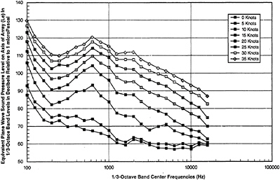
FIG. 25 MEASURED COMPOSITE ARRAY SELF-NOISE (Le) VERSUS SPEED FOR AN EMPTY TUNNEL

FIG. 26 ARL PENN STATE 48-INCH DIAMETER WATER TUNNEL AND HIGH REYNOLDS NUMBER PUMP INSTALLATION
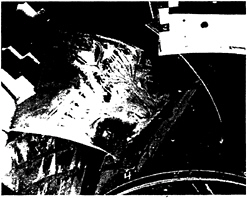
FIG. 27 INSTALLATION OF TRANSDUCERS ON BLADE
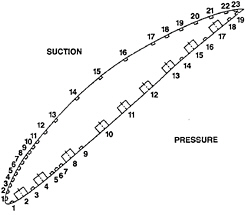
FIG. 28 SCHEMATIC OF PRESSURE TRANSDUCER AND ACCELEROMETER INSTALLATION
IN CONCLUSION
As in the past, today's propulsor designers still rely heavily on a combination of numerical and experimental inputs in order to meet powering, cavitation and acoustic requirements. Some time in the future it is reasonable to expect that supercomputers and physically correct descriptions of the flow and of structural responses will be capable of predicting all required performance parameters with confidence. A program aimed at achieving this objective would be a very ambitious and costly
undertaking. However, it would have a major payoff in saving design time, and the very high cost of experimental hardware and facilities. It would also provide “agility” to the ship design process, as rapid means for assessing the merits and limitations of various options will be at hand.
REFERENCES
1. Lighthill, M.J., “On Sound Generated Aerodynamically, I, General Theory.” Proc. R. Soc., London, Ser. A 211, 564–587 ( 1952).
2. Powell, A., “Theory of Vortex Sound.” J. Acoust. Soc. Am. 36, 177–195 ( 1964).
3. Ffowcs Williams, J.E., “Sound Radiation from Turbulent Boundary Layers Formed on Compliant Surfaces.” J. Fluid Mech. 22, 347–358 ( 1965).
4. Curle, N., “The Influence of Solid Boundaries upon Aerodynamic Sound.” Proc. R. Soc. London, Ser. A.231, 505–514 ( 1955).
5. Ffowcs Williams, J.E., “Modern Methods in Analytical Acoustics, Chapter 11”. Springer Verlag, ( 1994).
6. Blake, W.K., “Mechanics of Flow-Induced Sound and Vibration”. Academic Press, ( 1986).
7. Sevik, M., “The Response of Propulsors to Turbulence”. Seventh Symposium on Naval Hydrodynamics”. Office of Naval Research, DR.-148, 293–313 ( 1968).
8. Jiang, C.W., Chang, M.S., Liu, Y.N., “The Effect of Turbulence Ingestion on Propeller Broadband Thrust. ” David Taylor Model Basin, Report Number DTRC/SHD-1355–02, ( 1991).
9. Martinez, R., “Asymptotic Theory of Broadband Rotor Thrust; Parts I and II”. Cambridge Acoustical Associates, Inc. ( 1995).
10. Kim, S.K., “Radiation of Sound by a Point-Excited Free-Flooded Cylindrical Shell of Finite Length”. David Taylor Model Basin, ( 1995).
11. Howe, M.S., “Production of Structural and Acoustic Waves by Dipole Sources Adjacent to an Elastic Plate with a Pressure-Release Coating”. J. Acoust. Soc. Am. 91 (3), ( 1992)


